White’s Reality Check

This is the third part of the Trend Experiment article series. We now want to evaluate if the positive results from the 900 tested trend following strategies are for real, or just caused by Data Mining Bias. But what is Data Mining Bias, after all? And what is this ominous White’s Reality Check?

Suppose you want to trade by moon phases. But you’re not sure if you shall buy at full moon and sell at new moon, or the other way around. So you do a series of moon phase backtests and find out that the best system, which opens positions at any first quarter moon, achieves 30% annual return. Is this finally the proof that astrology works?

A trade system based on a nonexisting effect has normally a profit expectancy of zero (minus trade costs). But you won’t get zero when you backtest variants of such a system. Due to statistical fluctuations, some of them will produce a positive and some a negative return. When you now pick the best performer, such as the first quarter moon trading system, you might get a high return and an impressive equity curve in the backtest. Sadly, its test result is not necessarily caused by clever trading. It might be just by clever selecting the random best performer from a pool of useless systems.

For finding out if the 30% return by quarter moon trading are for real or just the fool’s gold of Data Mining Bias, Halbert White (1959-2012) invented a test method in 2000.  White’s Reality Check (aka Bootstrap Reality Check) is explained in detail in the book ‘Evidence-Based Technical Analysis’ by David Aronson. It works this way:

1. Develop a strategy. During the development process, keep a record of all strategy variants that were tested and discarded because of their test results, including all abandoned algorithms, ideas, methods, and parameters. It does not matter if they were discarded by human decision or by a computer search or optimizing process.
2. Produce balance curves of all strategy variants, using detrended trade results and no trade costs. Note down the profit P of the best strategy.
3. Detrend all balance curves by subtracting the mean return per bar (not to be confused with detrending the trade results!). This way you get a series of curves with the same characteristics of the tested systems, but zero profit.
4. Randomize all curves by bootstrap with replacement. This produces new curves from the random returns of the old curves. Because the same bars can be selected multiple times, most new curves now produce losses or profits different from zero.
5. Select the best performer from the randomized curves, and note down its profit.
6.  Repeat steps 4 and 5 a couple 1000 times.
7. You now have a list of several 1000 best profits. The median M of that list is the Data Mining Bias by your strategy development process.
8. Check where the original best profit P appears in the list. The percentage of best bootstrap profits greater than P is the so-called p-Value of the best strategy. You want the p-Value to be as low as possible. If P is better than 95% of the best bootstrap profits, the best strategy has a real edge with 95% probability.
9. P minus M minus trade costs is the result to be expected in real trading the best strategy.

The method is not really intuitive, but mathematically sound. However, it suffers from a couple problems that makes WRC difficult to use  in real strategy development:

• You can see the worst problem already in step 1. During strategy development you’re permanently testing ideas, adding or removing parameters, or checking out different assets and time frames. Putting aside all discarded variants and producing balance curves of all combinations of them is a cumbersome process. It gets even more diffcult with machine learning algorithms that optimize weight factors and usually do not produce discarded variants. However, the good news are that you can easily apply the WRC when your strategy variants are produced by a transparent mechanical process with no human decisions involved. That’s fortunately the case for our trend experiment.
• WRC tends to type II errors. That means it can reject strategies although they have an edge. When more irrelevant variants – systems with random trading and zero profit expectancy – are added to the pool,  more positive results can be produced in steps 4 and 5, which reduces the probability that your selected strategy survives the test. WRC can determine rather good that a system is profitable, but can not as well determine that it is worthless.
• It gets worse when variants have a negative expectancy.  WRC can then over-estimate Data Mining Bias (see paper 2 at the end of the article). This could theoretically also happen with our trend systems, as some variants may suffer from a phase reversal due to the delay by the smoothing indicators, and thus in fact trade against the trend instead of with it.

The Experiment

First you need to collect daily return curves from all tested strategies. This requires adding a few lines to the Trend.c script from the previous article:

// some global variables
int Period;
var Daily[3000];
...
// in the run function, set all trading costs to zero
 Spread = Commission = RollLong = RollShort = Slippage = 0;
...
// store daily results in an equity curve
  Daily[Day] = Equity;
}
...
// in the objective function, save the curves in a file for later evaluation
string FileName = "Log\\TrendDaily.bin";
string Name = strf("%s_%s_%s_%i",Script,Asset,Algo,Period);
int Size = Day*sizeof(var); 
file_append(FileName,Name,strlen(Name)+1);
file_append(FileName,&Size,sizeof(int));
file_append(FileName,Daily,Size);

The second part of the above code stores the equity at the end of any day in the Daily array. The third part stores a string with the name of the strategy, the length of the curve,  and the equity values itself in a file named TrendDaily.bin in the Log folder. After running the 10 trend scripts, all 900 resulting curves are collected together in the file.

The next part of our experiment is the Bootstrap.c script that applies White’s Reality Check. I’ll write it in two parts. The first part just reads the 900 curves from the TrendDaily.bin file, stores them for later evaluation, finds the best one and displays a histogram of the profit factors. Once we got that, we did already 80% of the work for the Reality Check. This is the code:

void _plotHistogram(string Name,var Value,var Step,int Color)
{
  var Bucket = floor(Value/Step);
  plotBar(Name,Bucket,Step*Bucket,1,SUM+BARS+LBL2,Color);
}

typedef struct curve
{
  string Name;
  int Length;
  var *Values;
} curve;

curve Curve[900];
var Daily[3000];

void main()
{
  byte *Content = file_content("Log\\TrendDaily.bin");
  int i,j,N = 0;
  int MaxN = 0;
  var MaxPerf = 0.0;
	
  while(N<900 && *Content)
  {
// extract the next curve from the file
    string Name = Content;
    Content += strlen(Name)+1;
    int Size = *((int*)Content);
    int Length = Size/sizeof(var); // number of values
    Content += 4;
    var *Values = Content;
    Content += Size;

// store and plot the curve		
    Curve[N].Name = Name;
    Curve[N].Length = Length;
    Curve[N].Values = Values;
    var Performance = 1.0/ProfitFactor(Values,Length);
    printf("\n%s: %.2f",Name,Performance);
    _plotHistogram("Profit",Performance,0.005,RED);

// find the best curve		
    if(MaxPerf < Performance) {
      MaxN = N; MaxPerf = Performance;
    }
    N++;
  }
  printf("\n\nBenchmark: %s, %.2f",Curve[MaxN].Name,MaxPerf); 
}

Most of the code is just for reading and storing all the equity curves. The indicator ProfitFactor calculates the profit factor of the curve, the sum of all daily wins divided by the sum of all daily losses. However, here we need to consider the array order. Like many platforms, Zorro stores time series in reverse chronological order,  with the most recent data at the begin. However we stored the daily equity curve in straight chronological order. So the losses are actually wins and the wins actually losses, which is why we need to inverse the profit factor. The curve with the best profit factor will be our benchmark for the test.

This is the resulting histogram, the profit factors of all 900 (or rather, 705 due to the trade number minimum) equity curves:

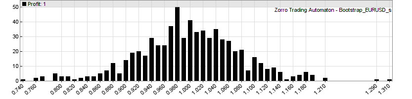
Note that the profit factors are slightly different to the parameter charts of the previous article because they were now calculated from daily returns, not from trade results. We removed trading costs, so the histogram is centered at a profit factor 1.0, aka zero profit. Only a few systems achieved a profit factor in the 1.2 range, the two best made about 1.3. Now we’ll see what White has to say to that. This is the rest of the main function in Bootstrap.c that finally applies his Reality Check:

plotBar("Benchmark",MaxPerf/0.005,MaxPerf,50,BARS+LBL2,BLUE);	
printf("\nBootstrap - please wait");
int Worse = 0, Better = 0;
for(i=0; i<1000; i++) {
  var MaxBootstrapPerf = 0;
  for(j=0; j<N; j++) {
    randomize(BOOTSTRAP|DETREND,Daily,Curve[j].Values,Curve[j].Length);
    var Performance = 1.0/ProfitFactor(Daily,Curve[j].Length);
    MaxBootstrapPerf = max(MaxBootstrapPerf,Performance);
  }
  if(MaxPerf > MaxBootstrapPerf)
    Better++;
  else
    Worse++;
  _plotHistogram("Profit",MaxBootstrapPerf,0.005,RED);
  progress(100*i/SAMPLES,0);
}
printf("\nBenchmark beats %.0f%% of samples!",
  (var)Better*100./(Better+Worse));

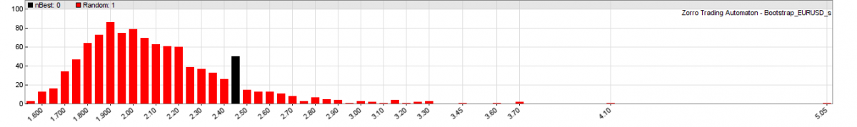
This code needs about 3 minutes to run; we’re sampling the 705 curves 1000 times. The randomize function will shuffle the daily returns by bootstrap with replacement; the DETREND flag tells it to subtract the mean return from all returns before. The number of random curves that are better and worse than the benchmark is stored, for printing the percentage at the end. The progress function moves the progress bar while Zorro grinds through the 705,000 curves. And this is the result:

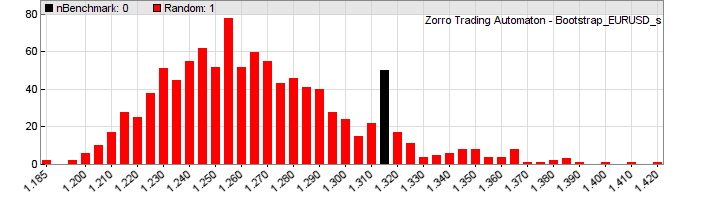
Hmm. We can see that the best system – the black bar – is at the right side of the histogram, indicating that it might be significant. But only with about 80% probability (the script gives a slightly different result every time due to the randomizing). 20% of the random curves achieve better profit factors than the best system from the experiment. The median of the randomized samples is about 1.26. Only the two best systems from the original distribution (first image) have profit factors above 1.26 – all the rest is at or below the bootstrap median.

So we have to conclude that this simple way of trend trading does not really work. Interestingly, one of those 900 tested systems is a system that I use for myself since 2012, although with additional filters and conditions. This system has produced good live returns and a positive result by the end of every year so far. And there’s still the fact that EUR/USD and silver in all variants produced better statistics than S&P500. This hints that some trend effect exists in their price curves, but the profit factors by the simple algorithms are not high enough to pass White’s Reality Check. We need a better approach for trend exploitation. For instance, a filter that detects if trend is there or not. This will be the topic of the next article of this series. We will see that a filter can have a surprising effect on reality checks. Since we now have the Bootstrap script for applying White’s Reality Check, we can quickly do further experiments.

The Bootstrap.c script has been added to the 2015 script collection downloadable on the sidebar.

Conclusion

• None of the 10 tested low-lag indicators, and none of the 3 tested markets shows significant positive expectancy with trend trading.
• There is evidence of a trend effect in currencies and commodities, but it is too weak or too infrequent for being effectively exploited with simple trade signals by a filtered price curve.
• We have now a useful code framework for comparing indicators and assets, and for further experiments with trade strategies.

Papers

1. Original paper by Dr. H. White:  White2000
2. WRC modification by P. Hansen: Hansen2005
3. Stepwise WRC Testing by J. Romano, M. Wolf: RomanoWolf2005
4. Technical Analysis examined with WRC, by P. Hsu, C. Kuan: HsuKuan2006
5. WRC and its Extensions by V. Corradi, N. Swanson: CorradiSwanson2011