
Most trading systems are of the get-rich-quick type. They exploit temporary market inefficiencies and aim for annual returns in the 100% area. They require regular supervision and adaption to market conditions, and still have a limited lifetime. Their expiration is often accompanied by large losses. But what if you’ve nevertheless collected some handsome gains, and now want to park them in a more safe haven? Put the money under the pillow? Take it into the bank? Give it to a hedge funds? Obviously, all that goes against an algo trader’s honor code. Here’s an alternative.
The old-fashioned investing method is buying some low-risk stocks and then waiting a long time. Any portfolio of stocks has a certain mean return and a certain fluctuation in value; you normally want to minimize the latter and maximize the former. Since the mean return and the fluctuation changes all the time, this task requires rebalancing the portfolio in regular intervals. The optimal capital allocation among the portfolio components produces either maximum mean return for a given allowed risk, or minimum risk – respectively, minimum variance – for a given mean return. This optimal allocation is often very different to investing the same amount in all N components of the portfolio. An easy way to solve this mean / variance optimization problem was published 60 years ago by Harry Markowitz. It won him later the Nobel prize.
The unfashionable Markowitz
Unfortunately, Markowitz got largely out of fashion since then. The problem is the same as with all trading algorithms: You can only calculate the optimal capital allocation in hindsight. Optimized portfolios mysteriously failed in live trading. They were said to often return less than a simple 1/N capital distribution. But this was challenged recently in an interesting paper (1) by Keller, Butler, and Kipnis, of which I quote the first paragraph:
Mean-Variance Optimization (MVO) as introduced by Markowitz (1952) is often presented as an elegant but impractical theory. MVO is an “unstable and error-maximizing” procedure (Michaud 1989), and is “nearly always beaten by simple 1/N portfolios” (DeMiguel, 2007). And to quote Ang (2014): “Mean-variance weights perform horribly… The optimal mean-variance portfolio is a complex function of estimated means, volatilities, and correlations of asset returns. There are many parameters to estimate. Optimized mean-variance portfolios can blow up when there are tiny errors in any of these inputs…”.
The optimized portfolios of the quoted authors indeed blew up. But Markowitz is not to blame. They just did not understand what ‘optimal capital allocation’ means. Suppose you have a portfolio of very similar assets, all with almost identical mean return and variance, only one of them is a tiny bit better. The Markowitz algorithm will then tend to assign all capital to that single asset. That’s just logical, as it is the optimal capital allocation. But it’s not the optimal portfolio. You don’t want to expose all capital to a single stock. If that company goes belly up, your portfolio will too. This is the mentioned ‘stability problem’. However there is a simple and obvious solution: a per-asset weight limit.
Aside from that, the Markowitz vituperators used too long, mean-reverting time periods for sampling the returns and covariances, and they applied the MVO algorithm wrongly to mixed long/short portfolios. When correctly applied to a momentum-governed time period and long-only, well diversified portfolios with a weight limit, MVO produced out of sample results far superior to 1/N. This was proven by testing a number of example portfolios in (1) with a R MVO implementation by fellow blogger Ilya Kipnis.
However, a R implementation is not very practical for live trading. For this we have to implement MVO in a real trade platform. Then we can park our money in an optimized portfolio of stocks and ETFs, let the platform rebalance the capital allocation in regular intervals, lean back, wait, and get rich slowly.
Implementing MVO
The Zorro implementation is based on Markowitz’ 1959 publication (2). In chapter 8, he described the MVO algorithm in a clear and easy to follow way. For simple minded programmers like me, he even included a brief introduction to linear algebra! I only modified his original algorithm by adding the mentioned weight constraint. This constraint stabilizes the algorithm and keeps the portfolio diversified.
In wise anticipation of future computing machines, Markowitz also included an example portfolio for checking if you programmed his algorithm correctly. The proof:
function main()
{
	var Means[3] = { .062,.146,.128 };
	var Covariances[3][3] = {.0146,.0187,.0145,.0187,.0854,.0104,.0145,.0104,.0289};
	var Weights[3];

	var BestVariance = markowitz(Covariances,Means,3,0);

	markowitzReturn(Weights,1);
	printf("\nMax:  %.2f %.2f %.2f",Weights[0],Weights[1],Weights[2]);
	markowitzReturn(Weights,BestVariance);
	printf("\nBest: %.2f %.2f %.2f",Weights[0],Weights[1],Weights[2]);
	markowitzReturn(Weights,0);
	printf("\nMin:  %.2f %.2f %.2f",Weights[0],Weights[1],Weights[2]);
}
The means and covariances arrays in the script are from Markowitz’ example portfolio. The markowitz function runs the algorithm and returns the variance value associated with the best Sharpe ratio. The markowitzReturn function then calculates the capital allocation weights with the maximum mean return for a given variance. The weights for maximum, best, and minimum variance are printed. If I did it right, they should be exactly the same as in Markowitz’ publication:
Max:  0.00 1.00 0.00
Best: 0.00 0.22 0.78
Min:  0.99 0.00 0.01
Selecting the assets
For long-term portfolios you can’t use the same high-leverage Forex or CFD instruments that you preferred for your short-term strategies. Instead you normally invest in stocks, ETFs, or similar instruments. They offer several advantages for algo trading:
- No zero-sum game. In the long run, stocks and index ETFs have positive mean returns due to dividends and accumulated value, while Forex pairs and index CFDs have negative mean returns due to swap/rollover fees.
- Serious brokers. Stock/ETF brokers are all regulated, what can not be said of all Forex/CFD brokers.
- More data for your algorithms, such as volume and market depth information.
- Bigger choice of assets from many different market sectors.
- More trading methods, such as pairs trading (“stat arb”), trading risk-free assets such as T-bills, or trading volatility.
The obvious disadvantage is low leverage, like 1:2 compared with 1:100 or more for Forex instruments. Low leverage is ok for a long-term system, but not for getting rich quick. More restrictions apply to long-term portfolios. MVO obviously won’t work well with components that have no positive mean return. And it won’t work well either when the returns are strongly correlated. So when selecting assets for your long-term portfolio, you have to look not only for returns, but also for correlation. Here’s the main part of a Zorro script for that:
#define NN  30  // max number of assets

function run()
{
	BarPeriod = 1440;
	NumYears = 7;
	LookBack = 6*252; // 6 years

	string	Names[NN];
	vars	Returns[NN];
	var	Correlations[NN][NN];

	int N = 0;
	while(Names[N] = loop(
		"TLT","LQD","SPY","GLD","VGLT","AOK"))
	{
		if(is(INITRUN))
			assetHistory(Names[N],FROM_YAHOO);
		asset(Names[N]);
		Returns[N] = series((priceClose(0)-priceClose(1))/priceClose(1));
		if(N++ >= NN) break;
	}
	if(is(EXITRUN)) {
		int i,j;
		for(i=0; i<N; i++)
		for(j=0; j<N; j++)
			Correlations[N*i+j] =
				Correlation(Returns[i],Returns[j],LookBack);
		plotHeatmap("Correlation",Correlations,N,N);
		for(i=0; i<N; i++)
			printf("\n%i - %s: Mean %.2f%%  Variance %.2f%%",
				i+1,Names[i],
				100*annual(Moment(Returns[i],LookBack,1)),
				252*100*Moment(Returns[i],LookBack,2));
	}
}
The script first sets up some parameters, then goes into a loop over N assets. Here I’ve just entered some popular ETFs; for replacing them, websites such as etfdb.com give an overview and help searching for the optimal ETF combination.
In the initial run, the asset prices are downloaded from Yahoo. They are corrected for splits and dividends. The assetHistory function stores them as historical price data files. Then the assets are selected and their returns are calculated and stored in the Returns data series. This is repeated with all 1-day bars of a 7 years test period (obviously the period depends on since when the selected ETFs are available). In the final run the script prints the annual mean returns and variances of all assets, which are the first and second moments of the return series. The annual function and the 252 multiplication factor convert daily values to annual values. The results for the selected ETFs:
1 - TLT: Mean 10.75% Variance 2.29%
2 - LQD: Mean 6.46% Variance 0.31%
3 - SPY: Mean 13.51% Variance 2.51%
4 - GLD: Mean 3.25% Variance 3.04%
5 - VGLT: Mean 9.83% Variance 1.65%
6 - AOK: Mean 4.70% Variance 0.23%
The ideal ETF has high mean return, low variance, and low correlation to all other assets of the portfolio. The correlation can be seen in the correlation matrix that is computed from all collected returns in the above code, then plotted in a N*N heatmap:
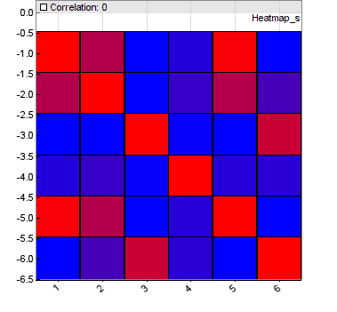
The correlation matrix contains the correlation coefficients of every asset with every other asset. The rows and columns of the heatmap are the 6 assets. The colors go from blue for low correlation between the row and column asset, to red for high correlation. Since any asset correlates perfectly with itself, we always have a red diagonal. But you can see from the other red squares that some of my 6 popular ETFs were no good choice. Finding the perfect ETF combination, with the heatmap as blue as possible, is left as an exercise to the reader.
The efficient frontier
After selecting the assets for our portfolio, we now have to calculate the optimal capital allocation, using the MVO algorithm. However, “optimal” depends on the desired risk, i.e. volatility of the portfolio. For every risk value there’s a optimal allocation that generates the maximum return. So the optimal allocation is not a point, but a curve in the return / variance plane, named the Efficient Frontier. We can calculate and plot it with this script:
function run()
{
	... // similar to Heatmap script

	if(is(EXITRUN)) {
		int i,j;
		for(i=0; i<N; i++) {
			Means[i] = Moment(Returns[i],LookBack,1);
			for(j=0; j<N; j++)
				Covariances[N*i+j] =
					Covariance(Returns[i],Returns[j],LookBack);
		}

		var BestV = markowitz(Covariances,Means,N,0);
		var MinV = markowitzVariance(0,0);
		var MaxV = markowitzVariance(0,1);

		int Steps = 50;
		for(i=0; i<Steps; i++) {
			var V = MinV + i*(MaxV-MinV)/Steps;
			var R = markowitzReturn(0,V);
			plotBar("Frontier",i,V,100*R,LINE|LBL2,BLACK);
		}
		plotGraph("Max Sharpe",(BestV-MinV)*Steps/(MaxV-MinV),
			100*markowitzReturn(0,BestV),SQUARE,GREEN);
	}
}
I’ve omitted the first part since it’s identical to the heatmap script. Only the covariance matrix is now calculated instead of the correlation matrix. Covariances and mean returns are fed to the markowitz function that again returns the variance with the best Sharpe ratio. The subsequent calls to markowitzVariance also return the highest and the lowest variance of the efficient frontier and establish the borders of the plot. Finally the script plots 50 points of the annual mean return from the lowest to the highest variance:
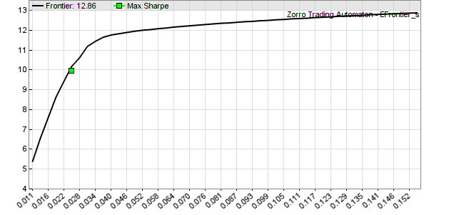
At the right side we can see that the portfolio reaches a maximum annual return of about 12.9%, which is simply all capital allocated to SPY. On the left side we achieve only 5.4% return, but with less than a tenth of the daily variance. The green dot is the point on the frontier with the best Sharpe ratio (= return divided by square root of variance) at 10% annual return and 0.025 variance. This is the optimal portfolio – at least in hindsight.
Experiments
How will a mean / variance optimized portfolio fare in an out of sample test, compared with with 1/N? Here’s a script for experiments with different portfolio compositions, lookback periods, weight constraints, and variances:
#define DAYS	252 // 1 year lookback period
#define NN	30  // max number of assets

function run()
{
	... // similar to Heatmap script

	int i,j;
	static var BestVariance = 0;
	if(tdm() == 1 && !is(LOOKBACK)) {
		for(i=0; i<N; i++) {
			Means[i] = Moment(Returns[i],LookBack,1);
			for(j=0; j<N; j++)
				Covariances[N*i+j] = Covariance(Returns[i],Returns[j],LookBack);
		}
		BestVariance = markowitz(Covariances,Means,N,0.5);
	}

	var Weights[NN];
	static var Return, ReturnN, ReturnMax, ReturnBest, ReturnMin;
	if(is(LOOKBACK)) {
		Month = 0;
		ReturnN = ReturnMax = ReturnBest = ReturnMin = 0;
	}

	if(BestVariance > 0) {
		for(Return=0,i=0; i<N; i++) Return += (Returns[i])[0]/N; // 1/N
		ReturnN = (ReturnN+1)*(Return+1)-1;

		markowitzReturn(Weights,0);	// min variance
		for(Return=0,i=0; i<N; i++) Return += Weights[i]*(Returns[i])[0];
		ReturnMin = (ReturnMin+1)*(Return+1)-1;

		markowitzReturn(Weights,1);	// max return
		for(Return=0,i=0; i<N; i++) Return += Weights[i]*(Returns[i])[0];
		ReturnMax = (ReturnMax+1)*(Return+1)-1;

		markowitzReturn(Weights,BestVariance); // max Sharpe
		for(Return=0,i=0; i<N; i++) Return += Weights[i]*(Returns[i])[0];
		ReturnBest = (ReturnBest+1)*(Return+1)-1;

		plot("1/N",100*ReturnN,AXIS2,BLACK);
		plot("Max Sharpe",100*ReturnBest,AXIS2,GREEN);
		plot("Max Return",100*ReturnMax,AXIS2,RED);
		plot("Min Variance",100*ReturnMin,AXIS2,BLUE);
	}
}
The script goes through 7 years of historical data, and stores the daily returns in the Returns data series. At the first trading day of every month (tdm() == 1) it computes the means and the covariance matrix of the last 252 days, then calculates the efficient frontier. This time we also apply a 0.5 weight constraint to the minimum variance point. Based on this efficient frontier, we compute the daily total return with equal weights (ReturnN), best Sharpe ratio (ReturnBest), minimum variance (ReturnMin) and maximum Return (ReturnMax). The weights remain unchanged until the next rebalancing, this way establishing an out of sample test. The four daily returns are added up to 4 different equity curves :
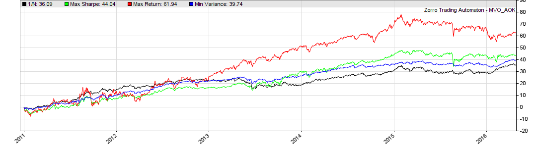
We can see that MVO improves the portfolio in all three variants, in spite of its bad reputation. The black line is the 1/N portfolio with equal weights for all asset. The blue line is the minimum variance portfolio – we can see that it produces slightly better profits than 1/N, but with much lower volatility. The red line is the maximum return portfolio with the best profit, but high volatility and sharp drawdowns. The green line, the maximum Sharpe portfolio, is somewhere inbetween. Different portfolio compositions can produce a different order of lines, but the blue and green lines have almost always a much better Sharpe ratio than the black line. Since the minimum variance portfolio can be traded with higher leverage due to the smaller drawdowns, it often produces the highest profits.
For checking the monthly rebalancing of the capital allocation weights, we can display the weights in a heatmap:
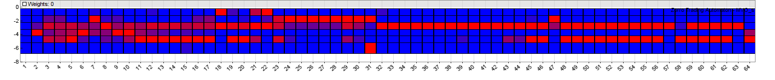
The horizontal axis is the month of the simulation, the vertical axis the asset number. High weights are red and low weights are blue. The weight distribution above is for the maximum Sharpe portfolio of the 6 ETFs.
The final money parking system
After all those experiments we can now code our long-term system. It shall work in the following way:
- The efficient frontier is calculated from daily returns of the last 252 trading days, i.e. one year. That’s a good time period for MVO according to (1), since most ETFs show 1-year momentum.
- The system rebalances the portfolio once per month. Shorter time periods, such as daily or weekly rebalancing, showed no advantage in my tests, but reduced the profit due to higher trading costs. Longer time periods, such as 3 months, let the system deteriorate.
- The point on the efficient frontier can be set up with a slider between minimum variance and maximum Sharpe. This way you can control the risk of the system.
- We use a 50% weight constraint at minimum variance. It’s then not anymore the optimal portfolio, but according to (1) – and my tests have confirmed this – it often improves the out of sample balance due to better diversification.
Here’s the script:
#define LEVERAGE 4	// 1:4 leverage
#define DAYS	252 	// 1 year
#define NN	30	// max number of assets

function run()
{
	BarPeriod = 1440;
	LookBack = DAYS;

	string Names[NN];
	vars	Returns[NN];
	var	Means[NN];
	var	Covariances[NN][NN];
	var	Weights[NN];

	var TotalCapital = slider(1,1000,0,10000,"Capital","Total capital to distribute");
	var VFactor = slider(2,10,0,100,"Risk","Variance factor");

	int N = 0;
	while(Names[N] = loop(
		"TLT","LQD","SPY","GLD","VGLT","AOK"))
	{
		if(is(INITRUN))
			assetHistory(Names[N],FROM_YAHOO);
		asset(Names[N]);
		Returns[N] = series((priceClose(0)-priceClose(1))/priceClose(1));
		if(N++ >= NN) break;
	}

	if(is(EXITRUN)) {
		int i,j;
		for(i=0; i<N; i++) {
			Means[i] = Moment(Returns[i],LookBack,1);
			for(j=0; j<N; j++)
				Covariances[N*i+j] = Covariance(Returns[i],Returns[j],LookBack);
		}
		var BestVariance = markowitz(Covariances,Means,N,0.5);
		var MinVariance = markowitzVariance(0,0);
		markowitzReturn(Weights,MinVariance+VFactor/100.*(BestVariance-MinVariance));

		for(i=0; i<N; i++) {
			asset(Names[i]);
			MarginCost = priceClose()/LEVERAGE;
			int Position = TotalCapital*Weights[i]/MarginCost;
			printf("\n%s:  %d Contracts at %.0f$",Names[i],Position,priceClose());
		}
	}
}
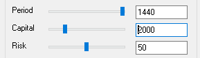
On Zorro’s panel you can set up the invested capital with a slider (TotalCapital) between 0 and 10,000$. A second slider (VFactor) is for setting up the desired risk from 0 to 100%: At 0 you’re trading with minimum variance, at 100 with maximum Sharpe ratio.
This script advises only, but does not trade: For automated trading it, you would need an API plugin to a ETF broker, such as IB. But the free Zorro version only has plugins for Forex/CFD brokers; the IB plugin is not free. However, since positions are only opened or closed once per month and price data is free from Yahoo, you do not really need an API connection for trading a MVO portfolio. Just fire up the above script once every month, and check what it prints out:
TLT:  0 Contracts at 129$
LQD:  0 Contracts at 120$
SPY:  3 Contracts at 206$
GLD:  16 Contracts at 124$
VGLT:  15 Contracts at 80$
AOK:  0 Contracts at 32$
Apparently, the optimal portfolio for this month consists of 3 contracts SPY, 16 contracts GLD, and 15 VGLT contracts. You can now manually open or close those positions in your broker’s trading platform until your portfolio matches the printed advice. Leverage is 4 by default, but you can change this to your broker’s leverage in the #define at the begin of the script. For a script that trades, simply replace the printf statement with a trade command that opens or closes the difference to the current position of the asset. This, too, is left as an exercise to the reader…
MVO vs. OptimalF
It seems natural to use MVO not only for a portfolio of many assets, but also for a portfolio of many trading systems. I’ve tested this with the Z12 system that comes with Zorro and contains about 100 different system/asset combinations. It turned out that MVO did not produce better results than Ralph Vince’s OptimalF factors that are originally used by the system. OptimalF factors do not consider correlations between components, but they do consider the drawdown depths, while MVO is only based on means and covariances. The ultimate solution for such a portfolio of many trading systems might be a combination of MVO for the capital distribution and OptimalF for weight constraints. I have not tested this yet, but it’s on my to do list.
I’ve added all scripts to the 2016 script repository. You’ll need Zorro 1.44 or above for running them. And after you made your first million with the MVO script, don’t forget to sponsor Zorro generously! 🙂
Papers
- Momentum and Markowitz – A Golden Combination: Keller.Butler.Kipnis.2015
- Harry M. Markowitz, Portfolio Selection, Wiley 1959
- MVO overview at guidedchoice.com
Markowitz seems not to be so “unfashionable” anymore, a couple papers came out about trading his algorithm in the last months. I’m going to test this concept. Thanks for this great article and the scripts!
Someone asked me how to prevent opening more than 4 positions at any time. For this you have to set all weights to zero, except for the 4 highest weights. I’m posting the code snippet here in case other people have the same question:
int* idx = sortIdx(Weights,N);var TotalWeight = 0;
for(i=N-4; i<N; i++) // sum up the 4 highest weights
TotalWeight += Weights[idx[i]];
for(i=0; i<N; i++) {
if(idx[i] < N-4)
Weights[i] = 0;
else // adjust weights so that their sum is still 1
Weights[i] /= TotalWeight;
}
Johann, are you going to publish an english edition of your book (Das Börsenhackerbuch: Finanziell unabhängig durch algorithmische Handelssysteme)?
Depends on demand. Besides, my English might be sufficient for a blog, but possibly not for a book.
Another outstanding contribution! What puzzles me a little bit is that the recently released Z8 system comes with a default set of assets that seems not to fulfill the “desperately” wanted lack of correlation. May be only a subset of four assets is uncorrelated. Some of the other assets have very substantial correlations as apparent from running the correlation heatmap script on the Z8 asset list. What has motivated this particular collection of assets?
Yes, the Z8 ETFs have been selected by fundamental considerations only, such as covering market sections with a positive perspective. They were not selected by their correlation. But you can replace them with any other assets if you want.
It’s actually a great and useful piece of information. I’m
satisfied that you just shared this useful information with us.
Please keep us up to date like this. Thanks for sharing.
amazing article. I added some etfs to the script but when i run it, it prints a negative number for some. e.g. TLT – 3 contracts at 139. Do you have any idea why this might be or how to fix it?
The number is calculated from Capital * Weight / MarginCost, and since neither of them is negative, the number shouldn’t either as I see it. Well, phenomena like this make programmer’s life interesting. If you have nothing changed with the script, let me know which assets you have added. When I get negative numbers too, I can most likely tell you their reason.
hey thanks jcl for the fast reply. that seems to be very odd. i am pretty new to programming/ trading, so i just added some of the assets from the z8 asset list.
i will just copy the asset part:
while(Names[N] = loop(
“TLT”,
“LQD”,
“SPY”,
“GLD”,
“VGLT”,
“AOK”,
“AGG”,
“DIA”,
“EWJ”,
“IVV”,
“IWM”,
“IYR”,
“KBE”,
“KRE”,
“LQD”,
“QQQ”,
“SMH”,
“SSO”,
“TLT”,
“VNQ”,
“XHB”,
“XLB”,
“XLF”,
“XLI”,
“XLK”,
“XLP”,
“XLU”,
“XLV”,
“XLY”,
“XRT”,
0))
… i didnt change the code besides that.
thanks in advance 🙂
oh i just saw that i have “TLT” twice in the list. I just removed one and now everything works fine!
Good, also make sure that when you have more than 30 assets, change the “NN” definition in the script to the maximum number of assets.
Hi Johann, does this work for stocks? BTW, how does one make use of the output? Let’s say I run the script now and it shows, AAPL: 3 Contracts at 114$. The price for 1 unit of AAPL now is 112.99$. Does it mean, if I don’t have any position on AAPL, I can buy it at 112.99$ and wait for it to hit 114$ before I close it or shall I wait for the price to hit 114$ before I buy? I think the former makes more sense. Thanks.
Yes, this also works for stocks, however they have higher volatility than ETFs, so you need more different stocks for diversification. You buy the position at market. The displayed price is only from the Yahoo history from the day before.
Hi Johann, thanks for the helpful reply. You mentioned that the script shall be run once a month to open or close a position. So let’s say I have a position on AAPL from previous month and when I run the script now and the output doesn’t show AAPL, does it mean I shall close it? Thanks.
Yes, exactly.
Hi Johann, thanks for the reply. I have compiled a list of stocks that I wanted to trade and there are about 100. In the code, I changed the array size, NN to 120 and included the 100 stocks however, the script run into run-time error that says, “Error 111: Crash in script: run()” and can’t proceed. Any idea? I am running Zorro 1.44 on Windows 7 64bit. Thanks.
If you changed NN to a large value, put also all arrays outside the function, or make them static. If I remember right, the default stack size is some 100 KB, so too large local arrays can exceed it.
Hi,
What is the difference between this scripts and Z8 script of Zorro strategy ?
Regards
I think there is no fundamental difference. Z8 is just a pimped version of this script.
I’m new(both for program and trading) and very interesting for this “Get Rich Slowly”. Could you mail me tell me how to create account and work with your system step by step?
And all about cost and studying time(normal).
Thanks! Happy new year!
If you’re new, the first step would be taking a trading and programming course. A short one can be found in the Zorro manual, a more extensive course is offered by a fellow blogger, Robotwealth. You can register for his course “Algorithmic Trading Funddamentals” on the Zorro download page, http://zorro-project.com/download.php.
I don’t understand why you are using priceClose() to calculate returns.
You should use adjusted price for that purpose, shouldn’t you?
I didn’t find in Zorro any function performing priceAdjust, neither any comment on their manual, why?
Interesting that Zorro do not provide any build-in “return” function,
opposed to R which provides many.
Yes, prices in backtests should be and are adjusted when not otherwise mentioned. I used no “return” function in the script since I trusted the reader to recognize a return expression when seeing it.
What language is the script written in?
C
Hi jcl, I see you didn’t do WFO in this system, I guess it’s because that one year’s look back period and one month’s rebalance period have been the optimal. WFO doesn’t make any sense here, is it correct?
Thank you
Jeff
Hi jcl,
I add script below to your MVO script and expect to see an equity curve, but nothing happened, what I did wrong?
StartDate = 2010;
NumWFOCycles = 3;
Thank you.
Jeff
I suppose you must not set the “NumWFOCycles” variable. It’s for WFO only. Since there are no optimized parameters in the script, there is also no WFO.
Thank you for your prompt comment.
I can test Z8, get all metrics like AR, SR Monte Carlo etc. How can I do the same thing to MVO? I still need to grab a sense how its results look like before I put it into live trading. In ther word, how can I test MVO?
Best
Jeff
By entering and closing positions. Z8 does this, while the scripts here only plot the return curves.
I think we have three metrics here for asset candidates, mean, variance and correlation, which one you think is more important?
Neither. When looking at a single asset, mean divided by square root of variance is a more important metric than mean or variance alone. When looking at a portfolio, it’s total mean divided by square root of total variance.
How about correlations?
mean divided by square root of variance is similar to Sharp Ratio?
Yes, it’s the Sharpe Ratio aside from a constant factor. And the correlation is insofar important as it affects the total variance of a portfolio – lower correlation means lower total variance.
I replied a thread on forum about MVO, could you please check it out?
http://www.opserver.de/ubb7/ubbthreads.php?ubb=showflat&Number=464393#Post464393
Thank you.
Jeff
Unfortuntately my boss does not allow me to check out program code of more than 10 lines – at least not without demanding money. But whatever does not work with your code, you can easily find out with the debugger. Help yourself, so help you god. The procedure is described in the Zorro manual under “troubleshooting”.
That’s fine, I am ZorroS user, I will get your support team to look at it later, I guess they would do that as the 4 weeks email support.
You gave out 2 versions of MVOtest, when you calculate BestVariance, you use different weight cap, 0.5 for your original version and 5./N for the latter one, it seems a constant 5 divided by the number of the assets. If I have 50 assets, the biggest weight in only 10%. Did I understand correctly? Why is that? Diversifying?
Thank you.
Jeff
Yes. From our experiments so far, many assets and low weight caps are better than few assets and high weight caps.
When you say better, I guess you mean low variance, not necessarily high return or high Sharp Ratio, is it?
Thank you
In this case a better Sharpe ratio.
Do you think put some negative/inverse correlation asset, like VIX, into the AssetList is a good idea?
Only when it has positive expectancy, such as assets derived from stocks or indices. VIX probably not. Maybe XIV, which can rise to high levels, but might impose high risk.
Thank you, you’ve been helpful.
Jeff
Any metrics to measure overall correlation of all assets like mean divided by sqrt of the variance except the heatmap? It’s visual, not numeric.
There is no such metrics as to my knowledge, but you can easily invent some. For instance the sum of all elements of the correlation matrix divided by the number of elements.
Thank you for your reply.
If I find some new assets with higher mean/sqrt of the variance ratio than the existing one, should I just replace the old one with the new one right way? Or should we modify the assets list periodically? Like every year? Or we should not modify the asset list at all!
Have a good one!
By all means feel free to use other assets. From what I hear, most people use their own asset lists with the Z8 strategy, instead of the default assets.
Thank you for your reply but it’s not what I asked. I understand we can use other assets than AssetZ8, my question is: should we periodically, let’s say every year, update the assets list, using new assets with higher momentum, lower variance to replace the old ones which has been in the list. F.I., using TSLA, which is not in the list right now but with higher momentum and lower variance to replace GE, which has been in the list. Or we simple add the new ones to the list, then we have a longer list.
Hopefully I made this clearly.
Best
Jeff
I understand your question, but that is completely up to you and the performance of the system. If an asset performs spectacularly bad, or if you got bad news about it, remove or replace it. Or if you encounter some promising new assets, add them. The system just determines the optimal portfolio weights. Aside from trading costs there is no particular disadvantage in adding or removing assets.
Hi Johann. Thanks for posting the wonderful articles. I enjoyed reading all of them. The backtest performance of the Z8 strategy is remarkable, with very little drawdowns. I tested the open script you included in this blog using the same 24 ETFs as in the Z8 strategy. But the results are not nearly as good as Z8. You mentioned in an earlier post that Z8 is just a pimped-up version of the script. Would you mind shedding more light on the major differences between the two? Thank you very much!
Z8 is a bit optimized. AFAIK it uses a 150 days lookback period for faster adaption, and a position on the EF very close to minimum variance. Also the weight cap is 4/number of assets.
Thank you for your reply, Johann. After more testing, I found that the Covariance() function in Zoro is defined as Sum((X_i – X_mean)*(Y_i – Y_mean)). Conventionally, covariance is defined as the Sum divided by (LookBack-1). Because the difference is just a scaling matter, it should not affect the backtest performance with the same parameters. But when I tested the code with the modified definition, Cov = Covaraince()/(LookBack-1), the backtest performance looks quite different. Can you please look in it? Thank you very much!
I can not see a difference with the MVOTest script when I multiply the covariance with a factor or divide them by Lookback-1. With which test did you get a difference?
I meant the last script included in your article. I think there may be a small typo in the script. Should the line “var MinVariance = markowitzReturn(0,0);” be “var MinVariance = markowitzVariance(0,0);” instead? Thanks!
Indeed! Thanks for the info. I’ve fixed the wrong line.
Within the delivered 2016 markowitz-scripts the compiler gives errors
“invalid number of arguments” function markowitz()
I added a zero parameter… but I am not sure, whether its correct.
Yes, zero is correct. The release version had a Cap parameter added to the markowitz function. I’ll fix the script.
Why Zorro could not download from Yahoo? I tried a couple of times, but failed and gave out error code 056. I checked Yahoo, it looks fine. What’s going on there? It used to work very well.
Jeff
I tried to change “FROM_YAHOO” to “FROM_QUANTL”, but it does not work, can we use other online server and what’s the right way to do that?
Thank you
Look here: http://www.opserver.de/ubb7/ubbthreads.php?ubb=showflat&Number=465333#Post465333
Thank you, it’s working now.
You mentioned Z8 uses 150 day LookBack, can we use Optimize() to find out an optimal LookBack period? If we can, how?
Jeff
Sure, you can optimize it just as any other parameter. Set LookBack to the maximum period and optimize the period used for calculating the means and covariance matrix.
Hi Johann. Is it possible to modify the Markowitz() function to allow constraints on the maximum weight of each asset? If not, do you know of any good Quadratic Programming package written in C that you recommend to use with Zorro? Thank you!
Yes, the markowitz function also accepts a weight caps vector as last parameter.
http://manual.zorro-project.com/markowitz.htm
Hi, can I understand more about this line in the code?
ReturnBest = (ReturnBest+1)*(Return+1)-1;
What are the difference between this line and in the Zorro manual for the calculation of AR (Annual Return) in the section of performance analysis?
The result does vary.
The quoted line is calculating the current return by multiplying yesterday’s return with today’s gain. Zorro’s AR is a measure of strategy performance, it divides the total return by the sum of maximum drawdown and maximum margin.
Did a lot of work and coding of this in Python. Very much enjoyed Ilya’s paper. Having followed trends in the futures market for many years I was looking for something very different. Unfortunately this approach is TF thinly disguised. For my money I prefer inverse volatility weighting on a portfolio of “uncorrelated” ETFs. Unfortunately of course in recent years “uncorrelated” has become a bit of a nonsense in a crisis.
https://anthonyfjgarner.net/2017/05/23/the-minimum-variance-misnomer/
Yes, with long term returns for calculating portfolio weights, most algorithms end up with some sort of trend following, since trend is the main market inefficiency of long periods. For something very different, you have to switch to short term trading and exploit mean reversion or other market anomalies.
Not necessarily, I think. Perhaps certain carry trades perform a useful role in supplementing trend following. I am thinking of “carry trades” in this context as being trades which “earn” rather than speculate. Although as you point out equites “earn” through a combination of dividends + price performance driven by long term earnings growth.
But more specifically interest carry trades on currencies (although there is again perhaps a trend following element contrary to interest rate parity), roll premium on futures and premium selling with options. None of which, sadly, are risk free.
Actually, the problem with slow, long term systems is much the same as with short term stuff. Frankly. Nothing has much predictive power and what worked yesterday may well not work tomorrow. Look at what happened to Bill Dunn and JW Henry in the CTA sphere. Look at the shitty CTA returns of the past 5 years. Your article on HFT and arb is a much better bet with those who have the right skillset even though we both know HFT returns have been on the decline in the recent low vol environment over the past few years.
But as you point out, front running doesn’t require much prediction, nor does arbing. If you happen to have the many hundreds of thousands of dollars for the infrastructure.
as stated MVO is a potential for positive mean returns what type of rebalancing would be ideal if you run a portfolio of negative mean returns?
If you mean a portfolio for shorting, a possibility would be MVO applied to the inverse momentum. I haven’t had yet such a portfolio, so tests and experiments would be required.
Yes, exactly, for shorting. The idea is if you have a pairs trading strategy (or any strategy) that is capable of going long or short, how to properly allocate amongst a large set of pairs. So I presume you could potentially take the trades for these pairs, split them into Long and Short and then run MVO and the inverse momentum MVO to figure out how you should allocate to any particular trade. Hopefully that was clear.
hi could you may be tell us the source for the Markowitz’s example portfolio? Nice one though
You mean the portfolio with the 3 stocks? It’s from Markowitz’ book.
Johann,
I see that you are using the first moment to evaluate average returns. If I’m not mistaken, this is a simple average.
Wouldn’t a geometric average of returns be more appropriate here?
An extreme example: An asset returns +200%, +200%, -99%, and 200%. A simple average will calculate an amazing return of 125%, whereas a geometric average calculates a -73% return.
It seems that simple average of returns will tend to overrate volatile assets, whereas a geometric average return will always better reflect actual returns of the sample period.
I made a math error in my last comment – total return was -73%, but the geometric average of returns is -27.9%. If you return -27.9% four times, your total return is -73%.
You’re right, a geometric average would be better than the mean, especially when assets have extreme volatility. I used the mean simply because anyone used it for MVO – after all it’s named Mean-Variance Optimization. Try the geometric average, maybe this will improve the performance.
Johann,
I ran some tests, and I have some observations:
1) In terms of profits, your original simple average formula tended to be more profitable, per the modified MVOTest script.
2) The deviation of Geometric Means tend to be large when variance is large. I modified the Heatmap script, and here’s the log output (five years of lookback):
1 – TLT: GeoMean 8.58% Mean 9.68% Variance 2.01% M/GM = 1.1216
2 – LQD: GeoMean 4.87% Mean 5.26% Variance 0.73% M/GM = 1.0762
3 – SPY: GeoMean 8.45% Mean 10.35% Variance 3.45% M/GM = 1.2141
4 – GLD: GeoMean 7.08% Mean 8.04% Variance 1.78% M/GM = 1.1295
5 – VGLT: GeoMean 8.44% Mean 9.39% Variance 1.74% M/GM = 1.1072
6 – AOK: GeoMean 3.67% Mean 3.86% Variance 0.38% M/GM = 1.0526
In the right column, I checked to see how much larger the mean was than the geometric mean.
OK, one more, but with one year of lookback:
1 – TLT: GeoMean 39.01% Mean 42.29% Variance 4.71% M/GM = 1.0710
2 – LQD: GeoMean 11.96% Mean 13.52% Variance 2.79% M/GM = 1.1223
3 – SPY: GeoMean -0.87% Mean 4.19% Variance 9.90% M/GM = -4.7005
4 – GLD: GeoMean 33.22% Mean 35.16% Variance 2.91% M/GM = 1.0504
5 – VGLT: GeoMean 38.18% Mean 40.92% Variance 3.97% M/GM = 1.0609
6 – AOK: GeoMean 3.50% Mean 4.05% Variance 1.07% M/GM = 1.1556
Here, you can see a huge discrepancy between SPY’s geometric mean and simple mean. Also, TLT and VGLT were wildly profitable in lookback, so their means were somewhat close together despite high volatility.
I have a hypothesis that your script is more aggressive/”fearless” than mine (more emphasis on volatile assets), and it’s somehow reaping extra profit from it.
At this point, I’m mostly curious to know how the resulting sharpe ratios compare. Perhaps the geometric equity curves are less volatile? More research required.
For your reference, here’s the geometric average function:
// Geometric Average of Returns.
// Data input: relative returns, e.g. 0.12 for 12% return, -0.054 for -5.4% return, etc.
// len: Number of elements to be averaged.
var GeometricAvg(vars Data, int len){
len = max(1,len);
int i;
var scaleup = 1;
for(i=0;i<len;i++){
scaleup *= Data[i] + 1;
}
return pow(scaleup,((var)1)/len)-1;
}
JCL, would you be so kind to explain one line of code in the final script for a beginner?
Covariances[N*i+j] = Covariance(Returns[i],Returns[j],LookBack);
Why N*i+j? We declared Covariances[NN][NN] (NN defined 30) as two-dimensional array and here we use only one dimension and with strange math as Covariances[6*6+6].
Thank you in advance
Yes, Covariances[i][j] would also work. But it is a bit slower, because [N*i+j] stores all values at the begin of the array, which is more cache effective. And it also works with dynamic arrays, while [i][j] would not.
This is just from my game programming background. We game programmers use always one-dimensional arrays and always address them with [N*i+j] for gaining a few microseconds. But speed does not matter much for this system, so you can also use the conventional [i][j] addressing if you want.
I had trouble getting the code to work for the plotHeatmap in the “Selecting the Assets” section. Using Zorro 2.40.
Got it to work by adding
#include
at the top.
Also changed the second to last line from
100*annual(Moment(Returns[i],LookBack,1)),
to
252*100*Moment(Returns[i],LookBack,1),
Just passing this along in case any one else is stuck.