
Despite the many interesting features of options, private traders rarely take advantage of them (of course I’m talking here of serious options, not binary options). Maybe options are unpopular due to their reputation of being complex. Or because they are unsupported by most trading software. Or due to the price tags of the few options trading tools and of the historical data that you need for algorithmic trading. Whatever – we recently did several programming contracts for algorithmic options trading systems, and I was surprised that even simple systems seemed to produce relatively consistent profit. Especially selling options appears more lucrative than trading ‘conventional’ instruments. This article is the first one of a mini-series about earning money with algorithmic options trading.
Options 101
Options are explained on many websites and in many trading books, so here’s just a quick overview. An option is a contract that gives its owner the right to buy (call option) or sell (put option) a financial asset (the underlying) at a fixed price (the strike price) at or before a fixed date (the expiry date). If you sell short (write) an option, you’re taking the other side of the trade. So you can enter a position in 4 different ways:
Buy a call – pay for the right to buy the underlying.
Buy a put – pay for the right to sell the underlying.
Write a call – get paid for the obligation to sell the underlying.
Write a put – get paid for the obligation to buy the underlying.
And this with all possible combinations of strike prices and expiry dates.
The premium is the price that you pay or collect for buying or selling an option. It is far less than the price of the underlying stock. Major option markets are usually liquid, so you can anytime buy, write, or sell an option with any reasonable strike price and expiry date. If the current underlying price (the spot price) of a call option lies above the strike price, the option is in the money; otherwise it’s out of the money. The opposite is true for put options. In-the-money is good for the buyer and bad for the seller. Options in the money can be exercised and are then exchanged for the underlying at the strike price. The difference of spot and strike is the buyer’s profit and the seller’s loss. American style options can be exercised anytime, European style options only at expiration.
Out-of-the-money options can not be exercised, at least not at a profit. But they are not worthless, since they have still a chance to walk into the money before expiration. The value of an option depends on that chance, and can be calculated for European options from spot price, strike, expiry, riskless yield rate, dividend rate, and underlying volatility with the famous Black-Scholes formula. This value is the basis of the option premium. The real premium might deviate slightly dependent on supply, demand, and belief in the underlying’s future price.
By reversing the formula with an approximation process, the volatility can be calculated from the real premium. This implied volatility is how the market expects the underlying to fluctuate in the next time. The partial derivatives of the option value are the Greeks (Delta, Vega – don’t know what Greek letter that’s supposed to be – and Theta). They determine in which direction, and how strong, the value will change when a market parameter changes.
That’s all basic info needed for trading options. By the way, it’s interesting to compare the performances of strategies from trading books. While the forex or stock trading systems described in those books are mostly bunk and lose already in a simple backtest, it is not so with option systems. They often win in backtests. And this even though apparently almost no book author has really backtested his system. Are options trading book authors just more intelligent than other trading book authors? Maybe, but we’ll see that there is an alternative explanation.
Why trading options at all?
They are more complex and more difficult to trade, and you need a Nobel prize winning formula to calculate a value that otherwise would simply be a difference of entry and exit price. Despite all this, options offer many wonderful advantages over other financial instruments:
- High leverage. With $100 you can buy only a few shares, but options of several hundred shares.
- Controlled risk. A short position in a stock can wipe your account; positions in options can be clever combined to limit the risk in any desired way. And unlike a stop loss it’s a real risk limit.
- Additional dimensions. Stock profits just depend on rising or falling prices. Option profits can be achieved with rising volatility, falling volatility, prices moving in a range, out of a range, or almost any other imaginable price behavior.
- Fire and forget. Options expire, so you don’t need an algorithm for closing them (unless you want to sell or exercise them on special conditions). And you pay no exit commission for an expired option.
- Seller advantage. Due to the premium, options can still produce a profit to their seller even if the underlying moves in the wrong direction.
Hacker ethics requires that you not just claim something, but prove it. For getting familiar with options, let’s put the last claim, the seller advantage, to the test:
void run()
{
	BarPeriod = 1440;
	assetList("assetsIB");
	assetHistory("SPY",FROM_YAHOO|UNADJUSTED);
	asset("SPY");
	if(is(INITRUN)) dataLoad(1,"SPY_Options.t8",9);

	Multiplier = 100;
	contractUpdate("SPY",1,CALL|PUT);
	int Type = ifelse(random() > 0,CALL,PUT);
	contract(Type,30,priceClose());
	static int LastExpiry = 0;
	if(ContractType && LastExpiry != ContractExpiry) {
		enterShort();
		LastExpiry = ContractExpiry;
	}
}
This is a very simple option trading system. It randomly writes call or put options and keeps the positions open until they expire. Due to the put/call randomness it is trend agnostic. Before looking into code details, just run it in [Test] mode a couple times (you’ll need Zorro version 1.53 or above). You’ll notice that the result is different any time, but it is more often positive than negative, even though commission is subtracted from the profit. A typical outcome:
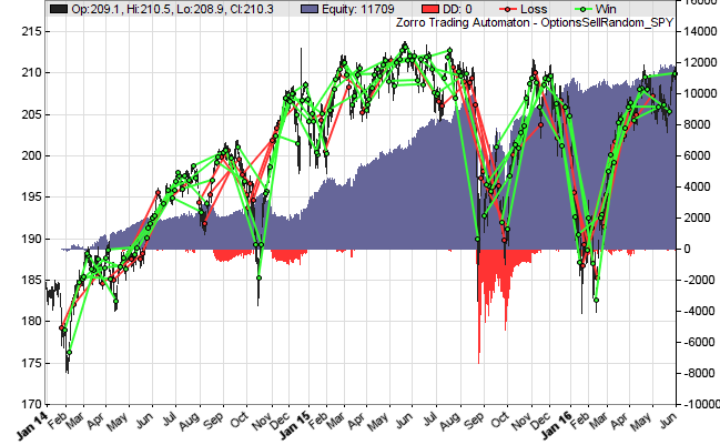
You can see that most trades win, but when they lose, they lose big. Now reverse the strategy and buy the options instead of selling them: Replace enterShort() by enterLong(). Run it again a couple times (the script needs about 3 seconds for a backtest). You will now see that the result is more often negative – in fact almost any time.
It seems that options, at least the tested SPY contracts, indeed favor the seller. This is somewhat similar to the positive expectancy of long positions in stocks, ETFs, or index futures, but the options seller advantage is stronger and independent of the market direction. It might explain a large part of the positive results of option systems in trading books. Why are there then option buyers at all? Options are often purchased not for profit, but as an insurance against unfavorable price trends of the underlying. And why is the seller advantage not arbitraged away by the market sharks? Maybe because there’s yet not much algorithmic trading with options, and because there are anyway more whales than sharks in the financial markets.
Functions for options
We can see that options trading and backtesting requires a couple more functions than just trading the underlying. Without options, the same random trading system would be reduced to this short script:
void run()
{
	BarPeriod = 1440;
	assetList("assetsIB");
	assetHistory("SPY",FROM_YAHOO);
	asset("SPY");

	if(random() > 0)
		enterLong();
	else
		enterShort();
}
Options require (at least) three additional functions:
- dataLoad(1,”SPY_Options.t8″,9) loads historical options data from the file “SPY_Options.t8” into a data set. Options data includes not only the ask and bid prices, but also the strike price, the expiration date, the type – put or call, American or European – of any option, and some rarely used additional data such as the open interest. Unlike historical price data, options data is usually expensive. You can purchase it from vendors such as iVolatility. But there’s an alternative way to get it for free, which I’ll describe below.
- contractUpdate(“SPY”,1,CALL|PUT) loads the current option chain. In backtest mode it’s loaded from the above data set, in live trading mode it’s loaded from the broker. The option chain is a list of all available option contracts of the selected underlying, with all available strike prices and all expiration dates. If you open it manually in the IB trading platform, it looks like this:
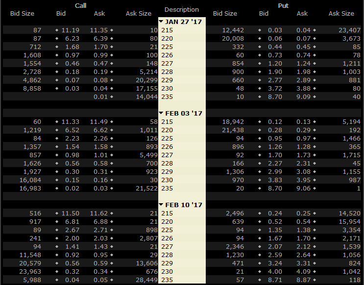
The center column lists different strike prices and expiry dates, the right and left parts are the ask and bid prices and order book sizes for their assigned call (left) and put options (right). The prices are per share; an option contract always covers a certain number of shares, normally 100. So you can see in the list above that you’ll collect $15 premium when you write a SPY call option expiring next week (Feb 03, 2017) with a $230 strike price. If SPY won’t rise above $230 until that date, the $15 are your profit. If it rised to $230 and 10 cents and the option is exercised (happens automatically when it expires in the money), you still keep $5. But if it suddenly soared to $300 (maybe Trump announced 100-ft. walls all around the US, all paid by himself), you have to bear a $6985 loss.
The image displays 54 contracts, but this is only a small part of the option chain, since there are many more expiry dates and strike prices available. The SPY option chain can contain up to 10,000 different options. They all are downloaded to the PC with the above contractUpdate function, which can thus take a couple seconds to complete.
- contract(Type,30,priceClose()) selects a particular option from the previously downloaded option chain. The type (PUT or CALL), the days until expiration (30), and the strike (priceClose() is the current price of the underlying) are enough information to select the best fitting option. Note that for getting correct strike prices in the backtest, we downloaded the underlying price data with the UNADJUSTED flag. Strike prices are always unadjusted.
Once a contract is selected, the next enterLong() or enterShort() buys or sells the option at market. The if() clause checks that the contract is available and its expiry date is different to the previous one (for ensuring that only different contracts are traded). Entry, stop, or profit limits would work as usual, they now only apply to the option value, the premium, instead of the underlying price. The backtest assumes that when an option is exercised or expires in the money, the underlying is immediately sold, and the profit is booked into the buyer’s account and deducted from the seller’s account. If the option expires out of the money, the position just vanishes. So we don’t care about exiting positions in this strategy. Apart from those differences, trading options works just as trading any other financial instrument.
Backtesting option strategies
Here’s an easy way to get rich. Open an IB account and run a software that records the options chains and contract prices in one-minute intervals. That’s what some data vendors did in the last 5 years, and now they are dear selling their data treasures. Although you can easily pay several thousand dollars for a few year’s option chains of major stocks, I am not sure who really owns the copyright of this data – the vendor, the broker, the exchange, or the market participants? This might be a legal grey area. Anyway, you need historical data for developing options strategies, otherwise you could not backtest them.
Here’s a method to get it for free and without any legal issues:
#include <contract.c>

string Code = "SPY";
string FileName = "History\\SPY_Options.t8";
var StrikeMax[3] = { 5,25,100 }; // strike ranges
var StrikeStep[3] = { 1,5,10 }; // strike step widths
int DaysMax = 180;  // max contract life in days
var BidAskSpread = 2.5; // bid/ask spread in percent
var Dividend = 2.0; // annual dividend in percent
int Type = 0; // or EUROPEAN, or FUTURE

/////////////////////////////////////////////////////////

CONTRACT* c;
int N = 0;

void run()
{
	BarPeriod = 1440;
	StartDate = 2011;
	EndDate = 2017;
	LookBack = 21;
	assetList("AssetsIB");
	assetHistory(Code,FROM_YAHOO|UNADJUSTED);
	asset(Code);
	if(is(INITRUN)) {
		initRQL();
		int MaxContractsPerDay = 2*(1+2*(StrikeMax[0]/StrikeStep[0] + StrikeMax[1]/StrikeStep[1] + StrikeMax[2]/StrikeStep[2])) * (1+DaysMax/7);
		int TotalContracts = (1+EndDate-StartDate)*252*MaxContractsPerDay;
		printf("\nAllocating %d Contracts",TotalContracts);
		c = (CONTRACT*)dataNew(1,TotalContracts,9);
		N = 0;
	}

	vars Close = series(priceClose());
	var HistVolOV = VolatilityOV(20);
	var Unl = Close[0];
	var Interest = yield();

	if(!is(LOOKBACK)) {
		var Strike;
		int i, Days = 1;
		while((dow()+Days)%7 != FRIDAY) Days++;
		for(; Days <= DaysMax; Days += 7)
		for(Strike = max(10,round(Unl-StrikeMax[2],StrikeStep[2])); Strike <= Unl+StrikeMax[2]; Strike)
		for(i = 0; i < 2; i++)
		{
			c->time = wdate();
			c->fUnl = Unl;
			c->fStrike = Strike;
			c->Type = Type | ifelse(i,PUT,CALL);
			c->Expiry = ymd(c->time+Days);
			c->fBid = contractVal(c,Unl,HistVolOV,0.01*Dividend,0.01*Interest);
			if(c->fBid < 0.01) continue; // probably no liquidity
			c->fAsk = (1.0+BidAskSpread/100)*c->fBid;

			if(abs(Unl-Strike) < StrikeMax[0]) Strike += StrikeStep[0];
			else if(abs(Unl-Strike) < StrikeMax[1]) Strike += StrikeStep[1];
			else Strike += StrikeStep[2];
			N++; c++;
		}
	}

	if(is(EXITRUN)) {
		printf("\nSaving %d Records",N);
		dataSort(1);	// reverse the entry order
		dataSave(1,FileName,0,N);
		printf("\nOk!");
	}
}
This script is a bit longer than the usual Zorro scripts that I post here, so I won’t explain it in detail. It generates artificial option chains for any day from 2011-2017, and stores them in a historical data file. The option prices are calculated from the underlying price, the volatility, the current risk free interest rate, and the dividend rate of the underlying. It uses three ranges of strike prices, and expiry dates at any Friday of the next 180 days. You need R installed for running it, and also the RQuantlib package for calculating option values. All functions are described in the Zorro manual. The yield() function returns the current yield rate of US treasury bills, and contractVal() calculates the premium by solving a differential equation with all option parameters. The source code of both functions can be found in the contract.c include file.
Due to the slow differential equation solver and the huge number of options, the script needs several hours to complete. Here’s a comparison of the generated data with real SPY options data:
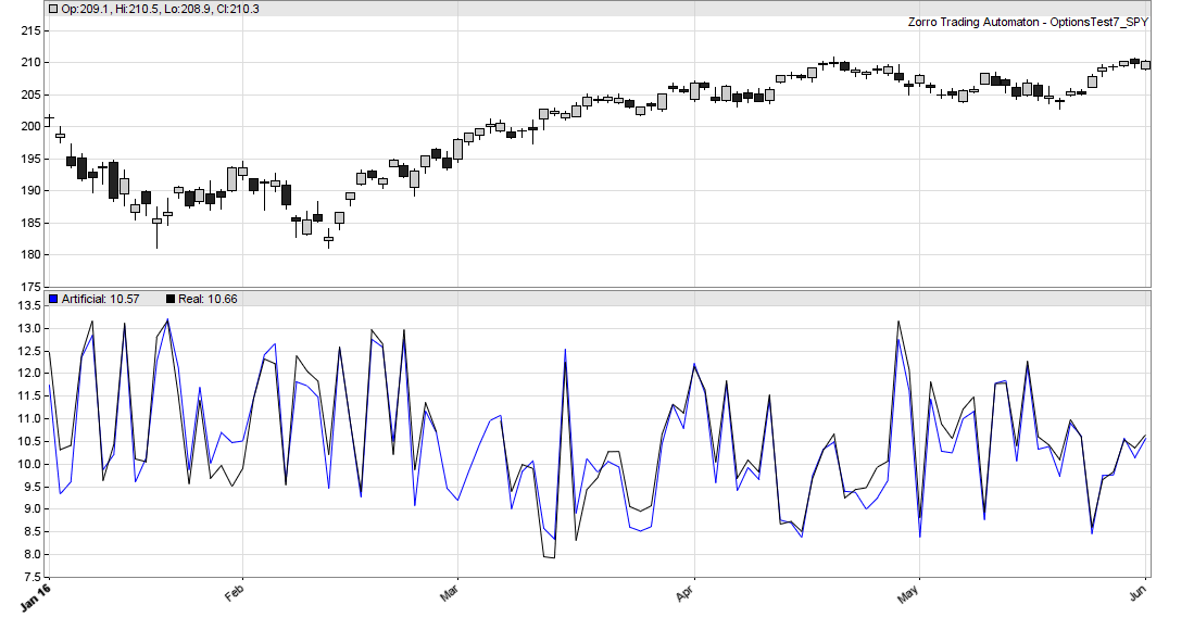
The blue line are the artificial option prices, the black line are the real prices purchased from an options data vendor, both for 3-weeks SPY contracts with 10 points spot-strike distance. You can see that the prices match quite well. There are some tiny differences that might be partially random, partially caused by anomalies in supply and demand. For strategies that exploit those anomalies – that includes all strategies based on implied volatility – you’ll need real historical options prices. For option strategies that exploit only price or volatility changes of the underlying, the artificial data will most likely do. See, reading this article up to the end already saved you a couple thousand dollars.
Conclusion
- Options and option combinations can be used to create artificial financial instruments with very interesting properties.
- Option strategies, especially options selling, are more likely to be profitable than other strategies.
- Algorithmic option strategies are a bit, but not much more complex than strategies with other financial instruments.
I’ve included all scripts in the 2017 script repository, and also a historical data set with the yield rates (otherwise you needed the Quandl bridge or Zorro S for downloading them). You’ll need Zorro 1.53 or above, which is currently available under the “Beta” link of the Zorro download page. The error message from the free Zorro version about the not supported Quandl bridge can be ignored, due to the included yield rates the script will run nevertheless.
In the next article we’ll look more closely into option values and into methods to combine options for limiting risk or trading arbitrary price ranges. Those combinations with funny names like “Iron Condor” or “Butterfly” are often referred to as option strategies, but they are not – they are just artificial financial instruments. How you trade them is up to the real strategy. Some simple, but consistently profitable option strategies will be the topic of the third article of this mini-series.
Very interesting article! I have one option automatic trading system created by Zorro developers (great job by the way) and it’s quite interesting to see, that my strategy generates similar results as your strategy “random”. I am looking forward for the next articles of this mini-series.
I would like to ask, do you have any idea if your book will be translated into English anytime soon? Would love to read the book.
I’m totally interested in this mini series articles. Please let me know the next one of the series.
My email is
andresortiz28@hotmail.com
Thanks – yes, an English book version is planned, I just must find some time for reviewing the raw translation. Andrés: you can enter your email in the subscribe field on the right.
Hi jcl,
Nice article, I would like to ask you what are good books or where I can learn to trade with options. Thanks
Am I right, rhat those artificial and real prices relate to a kind of a “synthetic” option made as a rolled-over series of real options with nearest expiration date and dynamically changed strike (depending on the underlying price)?
Investopedia and Tastytrade have some tutorials and videos about options. -It’s no rolled over series, but an option chain with different strikes and expiry dates, just as in real life. Otherwise the backtest would not be realistic.
When you’re comparing the artificial prices with the real prices, are you using ATM strike? The whole point, for me, of backtesting an option trading strategy vs. real option data is that at the wings the implied vols will be much much higher than those generated artificially.
The strikes used were about 10 points ITM.
Hi jcl,
Thanks for publishing this interesting article. May I know when the other two articles of this mini-series will be published?
Many thanks!
Regards,
Samer
When I get some time… 🙂
What a nice article! The results of the random trading system look similar to CBOE S&P 500 PutWrite Index and it makes sense.
Thank you so much for this article! Was just thinking about this the other day.
Hi jcl,
I like this blog’s articles very much. I am currently trading 1 year expiry call options of specific stocks.
My biggest problem with “seller advantage” that it contradicts to “controlled risk” statement.
http://www.investopedia.com/articles/optioninvestor/122701.asp
“Something that often confuses investors is whether or not being short a call and long a put are the same. Intuitively, this might make some sense, since calls and puts are almost opposite contracts, but being short a call and long a put are not the same. When you are long a put, you have to pay the premium and the worst case will result in a loss of only the premium. However, when you are short a call, you collect the option premium, but you are exposed to a large amount of risk”
So when you write (naked) calls your risk is unlimited. The short expiry time period(30 days) is saves you in most cases, but this is a self-delusion. This method is very similar to scam trading bots, where 99,5% of the time bots are winning little(e. g. call premium) amount of money, however when you loose, you risk large amount of your money.
Long call or put traders risk is limited and they choose out-of-the-money options to multiply their winnings and parallel they reduce their winning chance.
I would be interested in LEAPS (1+ year expiry long/put options) backtest.
Regards,
Tamas
Just do it. Download Zorro 1.54 from the user forum, and backtest a system with LEAPS. For this you need to increase the “DaysMax” variable in the options data generating script above to 1 year (365) or 2 years (2*365) for including long-term contracts. The script will then need a bit more time for the data generation.
Hi jcl,
Since trading options is a new Zorro feature, I’m wondering if the Broker API part of the manual (http://www.zorro-trader.com/manual/en/brokerplugin.htm) has been sufficiently updated to account for handling options.
I’m asking because I’m trying to write a DLL plugin for TradeKing (soon to be renamed to Ally Invest). They have stocks, ETFs, and options contracts. Very low barrier-to-entry broker as well ($0 required to get API access).
Thanks,
Andrew
For options, implement the basic API functions plus 5 BrokerCommand functions: GET_POSITION, GET_OPTIONS, GET_UNDERLYING, SET_SYMBOL, and SET_MULTIPLIER.
Aha! Thank you.
Johann,
Fantastic Article, thanks for sharing, I tried out the code and downloaded the options data via the script, it all seemed to download OK and make me a 48mb T8 file for SPY but when I run the random script I don’t get any trades. Its the first time I have ran zorro (I’m on the latest version downloaded 2-3 days ago) so really unsure what I’m doing wrong.
Any help would be appreciated and I really look forward to the next episode in this enthralling series 😉
Thanks
Michael
——————————————————————-
here is the log output:
Test OptionsSellRandom SPY
Simulated account AssetsIB
Bar period 24 hours (avg 2233 min)
Test period 12.01.2011-01.06.2016 (1270 bars)
Lookback period 80 bars (16 weeks)
Simulation mode Realistic (slippage 5.0 sec)
Spread 2.0 pips (roll 0.00/0.00)
Commission 0.02
Contracts per lot 1.0
Gross win/loss 0.00$ / -0.00$ (-1p)
Average profit 0.00$/year, 0.00$/month, 0.00$/day
Max drawdown -0.00$ -1% (MAE -0.00$ -1%)
Total down time 0% (TAE 0%)
Max down time 0 minutes from Sep 2010
Max open margin 0.00$
Max open risk 0.00$
Trade volume 0.00$ (0.00$/year)
Transaction costs 0.00$ spr, 0.00$ slp, 0.00$ rol
Capital required 0$
Number of trades 279 (52/year, 1/week, 1/day)
Percent winning 0.0%
Max win/loss 0.00$ / –0.00$
Avg trade profit 0.00$ -1.$p (+0.0p / -1.$p)
Avg trade slippage 0.00$ 1.$p (+0.0p / -1.$p)
Avg trade bars 23 (+0 / -23)
Max trade bars 26 (5 weeks)
Time in market 506%
Max open trades 6
Max loss streak 279 (uncorrelated 279)
Annual return 0%
Sharpe ratio 0.00
Kelly criterion 0.00
R2 coefficient 1.000
Ulcer index 0.0%
Confidence level AR DDMax Capital
10% 0% 1$ 1$
20% 0% 1$ 1$
30% 0% 1$ 1$
40% 0% 1$ 1$
50% 0% 1$ 1$
60% 0% 1$ 1$
70% 0% 1$ 1$
80% 0% 1$ 1$
90% 0% 1$ 1$
95% 0% 1$ 1$
100% 0% 1$ 1$
Portfolio analysis OptF ProF Win/Loss Wgt%
SPY .000 —- 0/279 -1.$
SPY:L .000 —- 0/0 -1.$
SPY:S .000 —- 0/279 -1.$
———————–
and a snippet of the log file…
[1338: Fri 13.05.16 19:00] +0 +0 6/271 (206.21)
[SPY::SC1272] Call 20160513 204.0 0@3.5713 not traded today!
[SPY::SC1272] Expired 1 Call 20160513 204.0 0@207: +0.00 at 19:00:00
[1339: Mon 16.05.16 19:00] +0 +0 5/272 (204.96)
[1340: Tue 17.05.16 19:00] +0 +0 5/272 (206.46)
[1341: Wed 18.05.16 19:00] +0 +0 5/272 (204.44)
[1342: Thu 19.05.16 19:00] +0 +0 5/272 (204.06)
[SPY::SC4278] Write 1 Call 20160624 205.0 0@3.4913 at 19:00:00
[1343: Fri 20.05.16 19:00] +0 +0 6/272 (204.92)
[SPY::SP1773] Put 20160520 208.0 0@4.2851 not traded today!
[SPY::SP1773] Expired 1 Put 20160520 208.0 0@204: +0.00 at 19:00:00
[1344: Mon 23.05.16 19:00] +0 +0 5/273 (205.51)
[1345: Tue 24.05.16 19:00] +0 +0 5/273 (206.17)
[1346: Wed 25.05.16 19:00] +0 +0 5/273 (208.67)
[1347: Thu 26.05.16 19:00] +0 +0 5/273 (209.44)
[SPY::SC4779] Write 1 Call 20160701 209.0 0@3.7358 at 19:00:00
[1348: Fri 27.05.16 19:00] +0 +0 6/273 (209.53)
[SPY::SP2274] Put 20160527 208.0 0@3.3622 not traded today!
[SPY::SP2274] Expired 1 Put 20160527 208.0 0@209: +0.00 at 19:00:00
[1349: Tue 31.05.16 19:00] +0 +0 5/274 (210.56)
[SPY::SC2775] Cover 1 Call 20160531 207.0 0@2.2309: +0.00 at 19:00:00
[SPY::SC3276] Cover 1 Call 20160531 205.0 0@5.1843: +0.00 at 19:00:00
[SPY::SP3777] Cover 1 Put 20160531 206.0 0@0.8602: +0.00 at 19:00:00
[SPY::SC4278] Cover 1 Call 20160531 205.0 0@4.9463: +0.00 at 19:00:00
[SPY::SC4779] Cover 1 Call 20160531 209.0 0@2.8347: +0.00 at 19:00:00
[1350: Wed 01.06.16 19:00] +0 +0 0/279 (209.12)
I see that the positions are all opened with zero volume, as if you had set the number of contracts to 0. Have you used the unmodified script from the repository?
I’m using the OptionsSimulate.c file straight from the Zip file.
I installed R and the Quantlib libraries and the R bridge seemed to work fine as well.
The top of the file
——————–
#include
string Code = “SPY”;
string FileName = “History\\SPY_SimOptions.t8”;
var StrikeMax[3] = { 5,30,80 }; // 3 strike ranges with different steps
var StrikeStep[3] = { 1,5,10 }; // stepwidths for the 3 ranges
int DaysMax = 180;
var BidAskSpread = 2.5; // Bid/Ask spread in percent
var Dividend = 0.02;
int Type = 0; // or EUROPEAN, or FUTURE
/////////////////////////////////////////////////////////
CONTRACT* c;
int N = 0;
void run()
{
BarPeriod = 1440;
StartDate = 2011;
EndDate = 2017;
LookBack = 21; // for volatility
assetList(“AssetsIB”);
assetHistory(Code,FROM_YAHOO|UNADJUSTED);
asset(Code);
……
I’m sorry for the n00b questions, its really interesting tools and systems and I was wanting to try out some vertical credit spreads using this code as a basis on the SPY and perhaps some other instruments!
Thanks
MB
It is not a noob question, it is in fact my fault. I just see that I’ve forgotten to set the options multiplier in the script. That did not matter with the previous Zorro version since the multiplier was 100 by default, but it must now be set because options can have very different multipliers.
Multiplier = 100;
I’ve corrected the script above. Thanks for notifying me!
Yes that was it!
Getting back results now, thanks so much for your help jcl.
I’m now off to put $1mm in an account and trade this baby 😉
Do you have any idea when you will get to work on the rest of the articles in this series?
Hi,
Looks like the code below is not working anymore
assetHistory(Code,FROM_YAHOO|UNADJUSTED); i
The CSV file SPY.csv get filled with this content:
QECx05,The url you requested is incorrect. Please use the following url instead: /api/v3/datasets/:database_code/:dataset_code.
Sorry, actually that file was from Quandl, and need a paid subscription.
From Yahoo I get the error Can’t download SPY from Yahoo.
Anyone having the same problem ?
Thanks
I guess all are having the same problem, as Yahoo changed their protocol last week. If you run into issues like that, look for a solution not only on my blog, but first on the Zorro forum:
http://www.opserver.de/ubb7/ubbthreads.php?ubb=showflat&Number=465333#Post465333
Thank you for this helpful information on automated trading systems!
I’m pretty new to this but I think this is a much bigger deal than you make it sound:
> There are some tiny differences that might be partially random, partially caused by anomalies in supply and demand. For strategies that exploit those anomalies you’ll need real historical data.
Having accurate volatility is essential. Without it, you’re not just writing a strategy that doesn’t exploit those anomalies, you’re writing one that totally ignores them. It’s comparable to generating a stock’s price by picking a random number based on the probability distribution of the previous weeks’ prices or smoothing out all the biggest moves.
Options prices are based on expectations about the future but (unless I misunderstand your code), you’re pricing them based on the past. The differences will be more pronounced on underlyings other than SPY, particularly around earnings time (say AAPL, MSFT or GOOG).
I also find it hard to think of a strategy that doesn’t exploit the difference between implied and actual volatility. Even a 16/5 delta put spread on SPY only works as well as it does because IV is much much higher than it should be.
Yes, option price changes due to expectation of volatility, maybe when company news approach, belongs to the mentioned anomalies. The general rule is: for anomalies that have also an effect on the underlying you can use the artificial prices. For anomalies that only affect options, but not the underlying, you’ll need to purchase real historical options data.
how good will the simulated data be if I will change BarPeriod =1440 to be BarPeriod = 1 ?
Theoretically, as good or bad as the daily data, since the priciple is the same. But I haven’t yet made tests with 1-minute options data. That’s an awful lot of data.
“Due to the slow differential equation solver and the huge number of options, the script needs several hours to complete.”
Yikes.
How much faster do you think this could be if the R / Quantmod stuff were replaced with C/C++? I’m thinking of generating lots of synthetic data.
I believe it _is_ C++, at least the underlying Quantlib is programmed in C++. The R overhead is probably negligible. The problem is not the code, but the math. Numerically solving differential equations is slow. Black-Scholes is much faster, but for European options only. If you have really lots of data to generate, it might make sense to check the speed of different approximation methods for American options.
I notice volatility is fixed at 20 in the above script for generating synthetic option prices. Might there not be an argument for volatility to be a rolling 30 days and calculated programatically from the underlying?
What do you mean with “a rolling 30 days”? 20 is the usual volatility period in financial calculations, since it is roughly equivalent to one month. 30 would probably not make much difference.
You use a one time estimate of Volatility I think: eg 16 for the S&P. But on a rolling basis it will very widely which is of course part of the reason why option prices change so much: as volatility rises so does the price of the option. If therefore you use a rolling 20 (or 30) day moving average of volatility you will obtain more accurate synthetic option prices than simply assuming a one time flat 16 for the S&P when sometimes actual might be 10 , sometimes 30. I have not looked at the architecture of zorro and so don’t now whether its mostly vector, or look or what. Either way it would be possible to include the relevant day’s moving average of the volatility of the underlying instrument rather than a fixed figure.
“vary widely”
But there again that is what you do perhaps? HistVolOV = VolatilityOV(20) – maybe this is 20 days? Not 20%?
A question not a statement
Anyway it looks a wonderful piece of software. Just going to plough my way through the manual.
Yep, looks like Vol is a time series. Sorry to bother you.
Yes, it’s annualized volatility from the last 20 days. If it were 20%, I would have written: HistVolOV = 0.2.
Nope. It doesn’t cut it. You can’t use a single measure of historic volatility for everything from a one month option to an expiry 24 months out. Perhaps the whole scheme is invalid. For instance IV for an SPX two year maturity is currently 15%+ while an option expiring in the next few days is 5% ish.
It may be invalid to use manufactured data at all. Except if you treat it as a sort of Monte Carlo test: this is what may/could have happened / might happen.
Anthony, the script is calculating the current price of an option. The current price depends on current volatility. Not on volatility from 24 months ago.
You calculate the value of European options with the Black Scholes formula, and American options, as in the script above, with an approximation method. Both methods normally use 20 days volatility. The volatility sampling method can differ, but the 20 days are pretty common to all options trading software that I know. And you can see from the comparison with real prices above that this period works rather well.
No, you can not calculate the current price of an option on any given day in that way. There is no way to accurately reproduce implied volatility hence price on any given date in the past. And it is the implied volatility we are interested in, not the historic. I totally agree on Black Scholes of course and its uses but it is cart before horse to expect to plug in 20 day volatility as at 3rd January 1985 and expect it to come up with an accurate price as traded at the close on that day for the SPX for any given strike or expiry.
It’s looking at it the wrong way around.
What you can try is to play around with different methods of estimating what the implied vol/ price MAY have been on 3rd Jan 1985 for a given strike and expiry of an SPX option.
For instance you might use 5 day historic volatility for an option expiring in a week and 252 day volatility for an option expiring in a year. Or you might imply volatilities by looking at the term structure of VIX futures contracts from 2004. Or at least use the VIX index itself going back to 1986 as input for 30 day volatility.
Whatever you do you won’t really be producing anything like what was actually traded on the day. Or at least not consistently and accurately over all expiries and strikes.
I believe that the process you describe does have a value but that the outcome of both the prices produced and the back tests resulting therefrom will be more akin to a random moet carlo process than to a back test on actual traded price data.
I believe it is a valuable process but that what is produced is a series of parallel universes: what might have happened to a given strategy over a given period of time using implied volatilities which may or may not have been traded.
Sorry to be long winded and I am an admirer of both your product and your script above. I would not have thought of generating fake option prices had I not seen your excellent article.
But in my opinion at least you need to rethink your input into the BS formula as far as volatility is concerned.
Incidentally please be well aware that I admire your product and your thoughts. Don’t imagine I am being difficult. Equally please don’t imagine I believe I am “right”!
I am just enjoying the journey and the dialogue with you and hoping together we can improve each other’s understanding of the topic.
Mine is limited!
Say the date you are looking atis 7th January 1987. On that day historic SPX volatility calculated over 20 trading days was 15.23. Historic volatility on that day for the past 252 days was 14.65
For 5 days it was 18
Now say I am trying to “calculate” (guess) a price (which might have been traded on 7th January 1987) for an option expiring in 5 days, 20 days and 252 days. Lets assume ATM.
My suspicion is that it would not be helpful to use 15.23 for all three expiries.
Thank you for your kind words. Finance is complex. My knowledge is even more limited and I’m daily surprised by some results that I didn’t expect. – In your example, the 15.23% volatility is the correct value. If you used a higher volatility period for higher expiration, then it depends on whether it’s still annualized volatility or just volatility of a longer time. In the latter case the results are off by some factor, in the former case they are based on too old volatility and thus not up to date. – You’re right about the implied volatility, since it is affected by the difference of theoretical and real option value. So you cannot use the script above for getting it. Otherwise you would just get back some approximation of the current volatility. You need real option prices for IV.
I hope that it’s alright that I discuss this with just a few of my clientele, this will assist
their knowledge of binary trading significantly.
What is your opinion on selling vertical spreads every month or two weeks in LEAPS? I’ve been interested in compiling historical SPY and QQQ returns monthly/daily for each year over the course of its inception and selling spreads at least 1+ years from expiration.
What is the best api broker for trading option ?
I would tell, but unfortunately that broker isn’t paying me enough.
Broker’s fees and margins are listed on their websites. Just compare.
Hi JCL I hope it’s not too far past the post date for you to see this question:
I downloaded the file, “FRED-DTBR.csv” and placed it in the History file for Zorro to attempt to generate the synthetic options data. I also tried changing the function to the “yieldCSV()” function so that it could grab the data directly from the csv file.
However, I’m still getting a syntax error when running the file with the code above to generate the data.
the error:
How can this be fixed?
Thanks a ton if you see this!
Syntax errors can be fixed by using correct syntax. There’s a chapter in the Zorro manual about fixing errors.
Hi JCL, in the simulated SPY.t8 data from the Zorro download page, the fields Val and VolDate are filled with non-zero values. I assume, these are the open interest and trade volume values. They are also simulated with this script OptionsSimulate.c ?
The options data on the Zorro download page is not simulated. It’s the real thing and has indeed OI and volume.
I had a thought for artificial options, and maybe I’ll develop it further in a blog post, but maybe there’s no need to generate the complete option history for certain types of trading systems. For example, if trading signals come entirely from the underlying price series only, then calculate option prices at select times. It’s probably a matter of manually managing a set of CONTRACT structs script-side. This can potentially save lots of time and disk space.