
Deep Blue was the first computer that won a chess world championship. That was 1996, and it took 20 years until another program, AlphaGo, could defeat the best human Go player. Deep Blue was a model based system with hardwired chess rules. AlphaGo is a data-mining system, a deep neural network trained with thousands of Go games. Not improved hardware, but a breakthrough in software was essential for the step from beating top Chess players to beating top Go players.
In this 4th part of the mini-series we’ll look into the data mining approach for developing trading strategies. This method does not care about market mechanisms. It just scans price curves or other data sources for predictive patterns. Machine learning or “Artificial Intelligence” is not always involved in data-mining strategies. In fact the most popular – and surprisingly profitable – data mining method works without any fancy neural networks or support vector machines.
Machine learning principles
A learning algorithm is fed with data samples, normally derived in some way from historical prices. Each sample consists of n variables x1 .. xn, commonly named predictors, features, signals, or simply input. These predictors can be the price returns of the last n bars, or a collection of classical indicators, or any other imaginable functions of the price curve (I’ve even seen the pixels of a price chart image used as predictors for a neural network!). Each sample also normally includes a target variable y, like the return of the next trade after taking the sample, or the next price movement. In the literature you can find y also named label or objective. In a training process, the algorithm learns to predict the target y from the predictors x1 .. xn. The learned ‘memory’ is stored in a data structure named model that is specific to the algorithm (not to be confused with a financial model for model based strategies!). A machine learning model can be a function with prediction rules in C code, generated by the training process. Or it can be a set of connection weights of a neural network.
Training: x1 .. xn, y => model
Prediction: x1 .. xn, model => y
The predictors, features, or whatever you call them, must carry information sufficient to predict the target y with some accuracy. They must also often fulfill two formal requirements. First, all predictor values should be in the same range, like -1 .. +1 (for most R algorithms) or -100 .. +100 (for Zorro or TSSB algorithms). So you need to normalize them in some way before sending them to the machine. Second, the samples should be balanced, i.e. equally distributed over all values of the target variable. So there should be about as many winning as losing samples. If you do not observe these two requirements, you’ll wonder why you’re getting bad results from the machine learning algorithm.
Regression algorithms predict a numeric value, like the magnitude and sign of the next price move. Classification algorithms predict a qualitative sample class, for instance whether it’s preceding a win or a loss. Some algorithms, such as neural networks, decision trees, or support vector machines, can be run in both modes.
A few algorithms learn to divide samples into classes without needing any target y. That’s unsupervised learning, as opposed to supervised learning using a target. Somewhere inbetween is reinforcement learning, where the system trains itself by running simulations with the given features, and using the outcome as training target. AlphaZero, the successor of AlphaGo, used reinforcement learning by playing millions of Go games against itself. In finance there are few applications for unsupervised or reinforcement learning. 99% of machine learning strategies use supervised learning.
Whatever signals we’re using for predictors in finance, they will most likely contain much noise and little information, and will be nonstationary on top of it. Therefore financial prediction is one of the hardest tasks in machine learning. More complex algorithms do not necessarily achieve better results. The selection of the predictors is critical to the success. It is no good idea to use lots of predictors, since this simply causes overfitting and failure in out of sample operation. Therefore data mining strategies often apply a preselection algorithm that determines a small number of predictors out of a pool of many. The preselection can be based on correlation between predictors, on significance, on information content, or simply on prediction success with a test set. Practical experiments with feature selection can be found in a recent article on the Robot Wealth blog.
Here’s a list of the most popular data mining methods used in finance.
1. Indicator soup
Most trading systems we’re programming for clients are not based on a financial model. The client just wanted trade signals from certain technical indicators, filtered with other technical indicators in combination with more technical indicators. When asked how this hodgepodge of indicators could be a profitable strategy, he normally answered: “Trust me. I’m trading it manually, and it works.”
It did indeed. At least sometimes. Although most of those systems did not pass a WFA test (and some not even a simple backtest), a surprisingly large number did. And those were also often profitable in real trading. The client had systematically experimented with technical indicators until he found a combination that worked in live trading with certain assets. This way of trial-and-error technical analysis is a classical data mining approach, just executed by a human and not by a machine. I can not really recommend this method – and a lot of luck, not to speak of money, is probably involved – but I can testify that it sometimes leads to profitable systems.
2. Candle patterns
Not to be confused with those Japanese Candle Patterns that had their best-before date long, long ago. The modern equivalent is price action trading. You’re still looking at the open, high, low, and close of candles. You’re still hoping to find a pattern that predicts a price direction. But you’re now data mining contemporary price curves for collecting those patterns. There are software packages for that purpose. They search for patterns that are profitable by some user-defined criterion, and use them to build a specific pattern detection function. It could look like this one (from Zorro’s pattern analyzer):
int detect(double* sig)
{
  if(sig[1]<sig[2] && sig[4]<sig[0] && sig[0]<sig[5] && sig[5]<sig[3] && sig[10]<sig[11] && sig[11]<sig[7] && sig[7]<sig[8] && sig[8]<sig[9] && sig[9]<sig[6])
      return 1;
  if(sig[4]<sig[1] && sig[1]<sig[2] && sig[2]<sig[5] && sig[5]<sig[3] && sig[3]<sig[0] && sig[7]<sig[8] && sig[10]<sig[6] && sig[6]<sig[11] && sig[11]<sig[9])
      return 1;
  if(sig[1]<sig[4] && eqF(sig[4]-sig[5]) && sig[5]<sig[2] && sig[2]<sig[3] && sig[3]<sig[0] && sig[10]<sig[7] && sig[8]<sig[6] && sig[6]<sig[11] && sig[11]<sig[9])
      return 1;
  if(sig[1]<sig[4] && sig[4]<sig[5] && sig[5]<sig[2] && sig[2]<sig[0] && sig[0]<sig[3] && sig[7]<sig[8] && sig[10]<sig[11] && sig[11]<sig[9] && sig[9]<sig[6])
      return 1;
  if(sig[1]<sig[2] && sig[4]<sig[5] && sig[5]<sig[3] && sig[3]<sig[0] && sig[10]<sig[7] && sig[7]<sig[8] && sig[8]<sig[6] && sig[6]<sig[11] && sig[11]<sig[9])
      return 1;
  ....
  return 0;
}
This C function returns 1 when the signals match one of the patterns, otherwise 0. You can see from the lengthy code that this is not the fastest way to detect patterns. A better method, used by Zorro when the detection function needs not be exported, is sorting the signals by their magnitude and checking the sort order. An example of such a system can be found here.
Can price action trading really work? Just like the indicator soup, it’s not based on any rational financial model. One can at best imagine that sequences of price movements cause market participants to react in a certain way, this way establishing a temporary predictive pattern. However the number of patterns is quite limited when you only look at sequences of a few adjacent candles. The next step is comparing candles that are not adjacent, but arbitrarily selected within a longer time period. This way you’re getting an almost unlimited number of patterns – but at the cost of finally leaving the realm of the rational. It is hard to imagine how a price move can be predicted by some candle patterns from weeks ago.
Still, a lot effort is going into that. A fellow blogger, Daniel Fernandez, runs a subscription website (Asirikuy) specialized on data mining candle patterns. He refined pattern trading down to the smallest details, and if anyone would ever achieve any profit this way, it would be him. But to his subscribers’ disappointment, trading his patterns live (QuriQuant) produced very different results than his wonderful backtests. If profitable price action systems really exist, apparently no one has found them yet.
3. Linear regression
The simple basis of many complex machine learning algorithms: Predict the target variable y by a linear combination of the predictors x1 .. xn.
[latex]y = a_0 + a_1 x_1 + … + a_n x_n[/latex]
The coefficients an are the model. They are calculated for minimizing the sum of squared differences between the true y values from the training samples and their predicted y from the above formula:
[latex]Minimize(\sum (y_i-\hat{y_i})^2)[/latex]
For normal distributed samples, the minimizing is possible with some matrix arithmetic, so no iterations are required. In the case n = 1 – with only one predictor variable x – the regression formula is reduced to
[latex]y = a + b x[/latex]
which is simple linear regression, as opposed to multivariate linear regression where n > 1. Simple linear regression is available in most trading platforms, f.i. with the LinReg indicator in the TA-Lib. With y = price and x = time it’s often used as an alternative to a moving average. Multivariate linear regression is available in the R platform through the lm(..) function that comes with the standard installation. A variant is polynomial regression. Like simple regression it uses only one predictor variable x, but also its square and higher degrees, so that xn == xn:
[latex]y = a_0 + a_1 x + a_2 x^2 + … + a_n x^n[/latex]
With n = 2 or n = 3, polynomial regression is often used to predict the next average price from the smoothed prices of the last bars. The polyfit function of MatLab, R, Zorro, and many other platforms can be used for polynomial regression.
4. Perceptron
Often referred to as a neural network with only one neuron. In fact a perceptron is a regression function like above, but with a binary result, thus called logistic regression. It’s not regression though, it’s a classification algorithm. Zorro’s advise(PERCEPTRON, …) function generates C code that returns either 100 or -100, dependent on whether the predicted result is above a threshold or not:
int predict(double* sig)
{
  if(-27.99*sig[0] + 1.24*sig[1] - 3.54*sig[2] > -21.50)
    return 100;
  else
    return -100;
}
You can see that the sig array is equivalent to the features xn in the regression formula, and the numeric factors are the coefficients an.
5. Neural networks
Linear or logistic regression can only solve linear problems. Many do not fall into this category – a famous example is predicting the output of a simple XOR function. And most likely also predicting prices or trade returns. An artificial neural network (ANN) can tackle nonlinear problems. It’s a bunch of perceptrons that are connected together in an array of layers. Any perceptron is a neuron of the net. Its output goes to the inputs of all neurons of the next layer, like this:
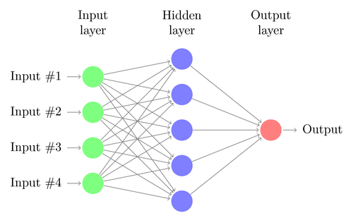
Like the perceptron, a neural network also learns by determining the coefficients that minimize the error between sample prediction and sample target. But this requires now an approximation process, normally with backpropagating the error from the output to the inputs, optimizing the weights on its way. This process imposes two restrictions. First, the neuron outputs must now be continuously differentiable functions instead of the simple perceptron threshold. Second, the network must not be too deep – it must not have too many ‘hidden layers’ of neurons between inputs and output. This second restriction limits the complexity of problems that a standard neural network can solve.
When using a neural network for predicting trades, you have a lot of parameters with which you can play around and, if you’re not careful, produce a lot of selection bias:
- Number of hidden layers
- Number of neurons per hidden layer
- Number of backpropagation cycles, named epochs
- Learning rate, the step width of an epoch
- Momentum, an inertia factor for the weights adaption
- Activation function
The activation function emulates the perceptron threshold. For the backpropagation you need a continuously differentiable function that generates a ‘soft’ step at a certain x value. Normally a sigmoid, tanh, or softmax function is used. Sometimes it’s also a linear function that just returns the weighted sum of all inputs. In this case the network can be used for regression, for predicting a numeric value instead of a binary outcome.
Neural networks are available in the standard R installation (nnet, a single hidden layer network) and in many packages, for instance RSNNS and FCNN4R.
6. Deep learning
Deep learning methods use neural networks with many hidden layers and thousands of neurons, which could not be effectively trained anymore by conventional backpropagation. Several methods became popular in the last years for training such huge networks. They usually pre-train the hidden neuron layers for achieving a more effective learning process. A Restricted Boltzmann Machine (RBM) is an unsupervised classification algorithm with a special network structure that has no connections between the hidden neurons. A Sparse Autoencoder (SAE) uses a conventional network structure, but pre-trains the hidden layers in a clever way by reproducing the input signals on the layer outputs with as few active connections as possible. Those methods allow very complex networks for tackling very complex learning tasks. Such as beating the world’s best human Go player.
Deep learning networks are available in the deepnet and darch R packages. Deepnet provides an autoencoder, Darch a restricted Boltzmann machine. I have not yet experimented with Darch, but here’s an example R script using the Deepnet autoencoder with 3 hidden layers for trade signals through Zorro’s neural() function:
library('deepnet', quietly = T)
library('caret', quietly = T)

# called by Zorro for training
neural.train = function(model,XY)
{
  XY <- as.matrix(XY)
  X <- XY[,-ncol(XY)] # predictors
  Y <- XY[,ncol(XY)]  # target
  Y <- ifelse(Y > 0,1,0) # convert -1..1 to 0..1
  Models[[model]] <<- sae.dnn.train(X,Y,
      hidden = c(50,100,50),
      activationfun = "tanh",
      learningrate = 0.5,
      momentum = 0.5,
      learningrate_scale = 1.0,
      output = "sigm",
      sae_output = "linear",
      numepochs = 100,
      batchsize = 100,
      hidden_dropout = 0,
      visible_dropout = 0)
}

# called by Zorro for prediction
neural.predict = function(model,X)
{
  if(is.vector(X)) X <- t(X) # transpose horizontal vector
  return(nn.predict(Models[[model]],X))
}

# called by Zorro for saving the models
neural.save = function(name)
{
  save(Models,file=name) # save trained models
}

# called by Zorro for initialization
neural.init = function()
{
  set.seed(365)
  Models <<- vector("list")
}

# quick OOS test for experimenting with the settings
Test = function()
{
  neural.init()
  XY <<- read.csv('C:/Project/Zorro/Data/signals0.csv',header = F)
  splits <- nrow(XY)*0.8
  XY.tr <<- head(XY,splits) # training set
  XY.ts <<- tail(XY,-splits) # test set
  neural.train(1,XY.tr)
  X <<- XY.ts[,-ncol(XY.ts)]
  Y <<- XY.ts[,ncol(XY.ts)]
  Y.ob <<- ifelse(Y > 0,1,0)
  Y <<- neural.predict(1,X)
  Y.pr <<- ifelse(Y > 0.5,1,0)
  confusionMatrix(Y.pr,Y.ob) # display prediction accuracy
}
7. Support vector machines
Like a neural network, a support vector machine (SVM) is another extension of linear regression. When we look at the regression formula again,
[latex]y = a_0 + a_1 x_1 + … + a_n x_n[/latex]
we can interpret the features xn as coordinates of a n-dimensional feature space. Setting the target variable y to a fixed value determines a plane in that space, called a hyperplane since it has more than two (in fact, n-1) dimensions. The hyperplane separates the samples with y > o from the samples with y < 0. The an coefficients can be calculated in a way that the distances of the plane to the nearest samples – which are called the ‘support vectors’ of the plane, hence the algorithm name – is maximum. This way we have a binary classifier with optimal separation of winning and losing samples.
The problem: normally those samples are not linearly separable – they are scattered around irregularly in the feature space. No flat plane can be squeezed between winners and losers. If it could, we had simpler methods to calculate that plane, f.i. linear discriminant analysis. But for the common case we need the SVM trick: Adding more dimensions to the feature space. For this the SVM algorithm produces more features with a kernel function that combines any two existing predictors to a new feature. This is analogous to the step above from the simple regression to polynomial regression, where also more features are added by taking the sole predictor to the n-th power. The more dimensions you add, the easier it is to separate the samples with a flat hyperplane. This plane is then transformed back to the original n-dimensional space, getting wrinkled and crumpled on the way. By clever selecting the kernel function, the process can be performed without actually computing the transformation.
Like neural networks, SVMs can be used not only for classification, but also for regression. They also offer some parameters for optimizing and possibly overfitting the prediction process:
- Kernel function. You normally use a RBF kernel (radial basis function, a symmetric kernel), but you also have the choice of other kernels, such as sigmoid, polynomial, and linear.
- Gamma, the width of the RBF kernel
- Cost parameter C, the ‘penalty’ for wrong classifications in the training samples
An often used SVM is the libsvm library. It’s also available in R in the e1071 package. In the next and final part of this series I plan to describe a trading strategy using this SVM.
8. K-Nearest neighbor
Compared with the heavy ANN and SVM stuff, that’s a nice simple algorithm with a unique property: It needs no training. So the samples are the model. You could use this algorithm for a trading system that learns permanently by simply adding more and more samples. The nearest neighbor algorithm computes the distances in feature space from the current feature values to the k nearest samples. A distance in n-dimensional space between two feature sets (x1 .. xn) and (y1 .. yn) is calculated just as in 2 dimensions:
[latex display=”true”]D = \sqrt{(x_1-y_1)^2 + (x_2-y_2)^2 + … + (x_n-y_n)^2}[/latex]
The algorithm simply predicts the target from the average of the k target variables of the nearest samples, weighted by their inverse distances. It can be used for classification as well as for regression. Software tricks borrowed from computer graphics, such as an adaptive binary tree (ABT), can make the nearest neighbor search pretty fast. In my past life as computer game programmer, we used such methods in games for tasks like self-learning enemy intelligence. You can call the knn function in R for nearest neighbor prediction – or write a simple function in C for that purpose.
9. K-Means
This is an approximation algorithm for unsupervised classification. It has some similarity, not only its name, to k-nearest neighbor. For classifying the samples, the algorithm first places k random points in the feature space. Then it assigns to any of those points all the samples with the smallest distances to it. The point is then moved to the mean of these nearest samples. This will generate a new samples assignment, since some samples are now closer to another point. The process is repeated until the assignment does not change anymore by moving the points, i.e. each point lies exactly at the mean of its nearest samples. We now have k classes of samples, each in the neighborhood of one of the k points.
This simple algorithm can produce surprisingly good results. In R, the kmeans function does the trick. An example of the k-means algorithm for classifying candle patterns can be found here: Unsupervised candlestick classification for fun and profit.
10. Naive Bayes
This algorithm uses Bayes’ Theorem for classifying samples of non-numeric features (i.e. events), such as the above mentioned candle patterns. Suppose that an event X (for instance, that the Open of the previous bar is below the Open of the current bar) appears in 80% of all winning samples. What is then the probability that a sample is winning when it contains event X? It’s not 0.8 as you might think. The probability can be calculated with Bayes’ Theorem:
[latex display=”true”]P(Y \vert X) = \frac{P(X \vert Y) P(Y)}{P(X)}[/latex]
P(Y|X) is the probability that event Y (f.i. winning) occurs in all samples containing event X (in our example, Open(1) < Open(0)). According to the formula, it is equal to the probability of X occurring in all winning samples (here, 0.8), multiplied by the probability of Y in all samples (around 0.5 when you were following my above advice of balanced samples) and divided by the probability of X in all samples.
If we are naive and assume that all events X are independent of each other, we can calculate the overall probability that a sample is winning by simply multiplying the probabilities P(X|winning) for every event X. This way we end up with this formula:
[latex display=”true”]P(Y | X_1 .. X_n) ~=~ s~P(Y) \prod_{i}{P(X_i | Y)}[/latex]
with a scaling factor s. For the formula to work, the features should be selected in a way that they are as independent as possible, which imposes an obstacle for using Naive Bayes in trading. For instance, the two events Close(1) < Close(0) and Open(1) < Open(0) are most likely not independent of each other. Numerical predictors can be converted to events by dividing the number into separate ranges.
The Naive Bayes algorithm is available in the ubiquitous e1071 R package.
11. Decision and regression trees
Those trees predict an outcome or a numeric value based on a series of yes/no decisions, in a structure like the branches of a tree. Any decision is either the presence of an event or not (in case of non-numerical features) or a comparison of a feature value with a fixed threshold. A typical tree function, generated by Zorro’s tree builder, looks like this:
int tree(double* sig)
{
  if(sig[1] <= 12.938) {
    if(sig[0] <= 0.953) return -70;
    else {
      if(sig[2] <= 43) return 25;
      else {
        if(sig[3] <= 0.962) return -67;
        else return 15;
      }
    }
  }
  else {
    if(sig[3] <= 0.732) return -71;
    else {
      if(sig[1] > 30.61) return 27;
      else {
          if(sig[2] > 46) return 80;
          else return -62;
      }
    }
  }
}
How is such a tree produced from a set of samples? There are several methods; Zorro uses the Shannon information entropy, which already had an appearance on this blog in the Scalping article. At first it checks one of the features, let’s say x1. It places a hyperplane with the plane formula x1 = t into the feature space. This hyperplane separates the samples with x1 > t from the samples with x1 < t. The dividing threshold t is selected so that the information gain – the difference of information entropy of the whole space, to the sum of information entropies of the two divided sub-spaces – is maximum. This is the case when the samples in the subspaces are more similar to each other than the samples in the whole space.
This process is then repeated with the next feature x2 and two hyperplanes splitting the two subspaces. Each split is equivalent to a comparison of a feature with a threshold. By repeated splitting, we soon get a huge tree with thousands of threshold comparisons. Then the process is run backwards by pruning the tree and removing all decisions that do not lead to substantial information gain. Finally we end up with a relatively small tree as in the code above.
Decision trees have a wide range of applications. They can produce excellent predictions superior to those of neural networks or support vector machines. But they are not a one-fits-all solution, since their splitting planes are always parallel to the axes of the feature space. This somewhat limits their predictions. They can be used not only for classification, but also for regression, for instance by returning the percentage of samples contributing to a certain branch of the tree. Zorro’s tree is a regression tree. The best known classification tree algorithm is C5.0, available in the C50 package for R.
For improving the prediction even further or overcoming the parallel-axis-limitation, an ensemble of trees can be used, called a random forest. The prediction is then generated by averaging or voting the predictions from the single trees. Random forests are available in R packages randomForest, ranger and Rborist.
Conclusion
There are many different data mining and machine learning methods at your disposal. The critical question: what is better, a model-based or a machine learning strategy? There is no doubt that machine learning has a lot of advantages. You don’t need to care about market microstructure, economy, trader psychology, or similar soft stuff. You can concentrate on pure mathematics. Machine learning is a much more elegant, more attractive way to generate trade systems. It has all advantages on its side but one. Despite all the enthusiastic threads on trader forums, it tends to mysteriously fail in live trading.
Every second week a new paper about trading with machine learning methods is published (a few can be found below). Please take all those publications with a grain of salt. According to some papers, phantastic win rates in the range of 70%, 80%, or even 85% have been achieved. Although win rate is not the only relevant criterion – you can lose even with a high win rate – 85% accuracy in predicting trades is normally equivalent to a profit factor above 5. With such a system the involved scientists should be billionaires meanwhile. Unfortunately I never managed to reproduce those win rates with the described method, and didn’t even come close. So maybe a lot of selection bias went into the results. Or maybe I’m just too stupid.
Compared with model based strategies, I’ve seen not many successful machine learning systems so far. And from what one hears about the algorithmic methods by successful hedge funds, machine learning seems still rarely to be used. But maybe this will change in the future with the availability of more processing power and the upcoming of new algorithms for deep learning.
Papers
- Classification using deep neural networks: Dixon.et.al.2016
- Predicting price direction using ANN & SVM: Kara.et.al.2011
- Empirical comparison of learning algorithms: Caruana.et.al.2006
- Mining stock market tendency using GA & SVM: Yu.Wang.Lai.2005
The next part of this series will deal with the practical development of a machine learning strategy.
Nice post. There is a lot of potential in these approach towards the market.
Btw are you using the code editor which comes with zorro? how is it possible to get such a colour configuration?
The colorful script is produced by WordPress. You can’t change the colors in the Zorro editor, but you can replace it with other editors that support individual colors, for instance Notepad++.
Thanks.
Is it then possible that notepad detects the zorro variables in the scripts? I mean that BarPeriod is remarked as it is with the zorro editor?
Theoretically yes, but for this you had to configure the syntax highlighting of Notepad++, and enter all variables in the list. As far as I know Notepad++ can also not be configured to display the function description in a window, as the Zorro editor does. There’s no perfect tool…
Concur with the final paragraph. I have tried many machine learning techniques after reading various ‘peer reviewed’ papers. But reproducing their results remains elusive. When I live test with ML I can’t seem to outperform random entry.
ML fails in live? Maybe the training of the ML has to be done with price data that include as well historical spread, roll, tick and so on?
I think reason #1 for live failure is data mining bias, caused by biased selection of inputs and parameters to the algo.
Thanks to the author for the great series of articles.
However, it should be noted that we don’t need to narrow our view with predicting only the next price move. It may happen that the next move goes against our trade in 70% of cases but it still worth making a trade. This happens when the price finally does go to the right direction but before that it may make some steps against us. If we delay the trade by one price step we will not enter the mentioned 30% of trades but for that we will increase the result of the remained 70% by one price step. So the criteria is which value is higher: N*average_result or 0.7*N*(avergae_result + price_step).
Nice post. If you just want to play around with some machine learning, I implemented a very simple ML tool in python and added a GUI. It’s implemented to predict time series.
http://algominr.com/release/algominr/
Thanks JCL I found very interesting your article. I would like to ask you, from your expertise in trading, where can we download reliable historical forex data? I consider it very important due to the fact that Forex market is decentralized.
Thanks in advance!
There is no really reliable Forex data, since every Forex broker creates their own data. They all differ slightly dependent on which liquidity providers they use. FXCM has relatively good M1 and tick data with few gaps. You can download it with Zorro.
Thanks for writing such a great article series JCL… a thoroughly enjoyable read!
I have to say though that I don’t view model-based and machine learning strategies as being mutually exclusive; I have had some OOS success by using a combination of the elements you describe.
To be more exact, I begin the system generation process by developing a ‘traditional’ mathematical model, but then use a set of online machine learning algorithms to predict the next terms of the various different time series (not the price itself) that are used within the model. The actual trading rules are then derived from the interactions between these time series. So in essence I am not just blindly throwing recent market data into an ML model in an effort to predict price action direction, but instead develop a framework based upon sound investment principles in order to point the models in the right direction. I then data mine the parameters and measure the level of data-mining bias as you’ve described also.
It’s worth mentioning however that I’ve never had much success with Forex.
Anyway, best of luck with your trading and keep up the great articles!
Thanks for posting this great mini series JCL.
I recently studied a few latest papers about ML trading, deep learning especially. Yet I found that most of them valuated the results without risk-adjusted index, i.e., they usually used ROC curve, PNL to support their experiment instead of Sharpe Ratio, for example.
Also, they seldom mentioned about the trading frequency in their experiment results, making it hard to valuate the potential profitability of those methods. Why is that? Do you have any good suggestions to deal with those issues?
ML papers normally aim for high accuracy. Equity curve variance is of no interest. This is sort of justified because the ML prediction quality determines accuracy, not variance.
Of course, if you want to really trade such a system, variance and drawdown are important factors. A system with lower accuracy and worse prediction can in fact be preferable when it’s less dependent on market condictions.
“In fact the most popular – and surprisingly profitable – data mining method works without any fancy neural networks or support vector machines.”
Would you please name those most popular & surprisingly profitable ones. So I could directly use them.
I was referring to the Indicator Soup strategies. For obvious reasons I can’t disclose details of such a strategy, and have never developed such systems myself. We’re merely coding them. But I can tell that coming up with a profitable Indicator Soup requires a lot of work and time.
Well, i am just starting a project which use simple EMAs to predict price, it just select the correct EMAs based on past performance and algorithm selection that make some rustic degree of intelligence.
Jonathan.orrego@gmail.com offers services as MT4 EA programmer.
Thanks for the good writeup. It in reality used to be a leisure account it.
Look complicated to more delivered agreeable from you!
By the way, how could we be in contact?
There are following issues with ML and with trading systems in general which are based on historical data analysis:
1) Historical data doesn’t encode information about future price movements
Future price movement is independent and not related to the price history. There is absolutely no reliable pattern which can be used to systematically extract profits from the market. Applying ML methods in this domain is simply pointless and doomed to failure and is not going to work if you search for a profitable system. Of course you can curve fit any past period and come up with a profitable system for it.
The only thing which determines price movement is demand and supply and these are often the result of external factors which cannot be predicted. For example: a war breaks out somewhere or other major disaster strikes or someone just needs to buy a large amount of a foreign currency for some business/investment purpose. These sort of events will cause significant shifts in the demand supply structure of the FX market . As a consequence, prices begin to move but nobody really cares about price history just about the execution of the incoming orders. An automated trading system can only be profitable if it monitors a significant portion of the market and takes the supply and demand into account for making a trading decision. But this is not the case with any of the systems being discussed here.
2) Race to the bottom
Even if (1) wouldn’t be true and there would be valuable information encoded in historical price data, you would still face following problem: there are thousands of gold diggers out there, all of them using similar methods and even the same tools to search for profitable systems and analyze the same historical price data. As a result, many of them will discover the same or very similar “profitable” trading systems and when they begin actually trading those systems, they will become less and less profitable due to the nature of the market.
The only sure winners in this scenario will be the technology and tool vendors.
I will be still keeping an eye on your posts as I like your approach and the scientific vigor you apply. Your blog is the best of its kind – keep the good work!
One hint: there are profitable automated systems, but they are not based on historical price data but on proprietary knowledge about the market structure and operations of the major institutions which control these markets. Let’s say there are many inefficiencies in the current system but you absolutely have no chance to find the information about those by analyzing historical price data. Instead you have to know when and how the institutions will execute market moving orders and front run them.
Thanks for the extensive comment. I often hear these arguments and they sound indeed intuitive, only problem is that they are easily proven wrong. The scientific way is experiment, not intuition. Simple tests show that past and future prices are often correlated – otherwise every second experiment on this blog had a very different outcome. Many successful funds, for instance Jim Simon’s Renaissance fund, are mainly based on algorithmic prediction.
One more thing: in my comment I have been implicitly referring to the buy side (hedge funds, traders etc) not to the sell side (market makers, banks). The second one has always the edge because they sell at the ask and buy at the bid, pocketing the spread as an additional profit to any strategy they might be running. Regarding Jim Simon’s Renaissance: I am not so sure if they have not transitioned over the time to the sell side in order to stay profitable. There is absolutely no information available about the nature of their business besides the vague statement that they are using solely quantitative algorithmic trading models…
Thanks for the informative post!
Regarding the use of some of these algorithms, a common complaint which is cited is that financial data is non-stationary…Do you find this to be a problem? Couldn’t one just use returns data instead which is (I think) stationary?
Yes, this is a problem for sure. If financial data were stationary, we’d all be rich. I’m afraid we have to live with what it is. Returns are not any more stationary than other financial data.
Hello sir, I developed some set of rules for my trading which identifies supply demand zones than volume and all other criteria. Can you help me to make it into automated system ?? If i am gonna do that myself then it can take too much time. Please contact me at svadukia@gmail.com if you are interested.
Sure, please contact my employer at info@opgroup.de. They’ll help.
I have noticed you don’t monetize your page, don’t waste your traffic,
you can earn extra bucks every month because you’ve got high quality content.
If you want to know how to make extra $$$, search for: Mrdalekjd methods for $$$
Technical analysis has always been rejected and looked down upon by quants, academics, or anyone who has been trained by traditional finance theories. I have worked for proprietary trading desk of a first tier bank for a good part of my career, and surrounded by those ivy-league elites with background in finance, math, or financial engineering. I must admit none of those guys knew how to trade directions. They were good at market making, product structures, index arb, but almost none can making money trading directions. Why? Because none of these guys believed in technical analysis. Then again, if you are already making your millions why bother taking the risk of trading direction with your own money. For me luckily my years of training in technical analysis allowed me to really retire after laying off from the great recession. I look only at EMA, slow stochastics, and MACD; and I have made money every year since started in 2009. Technical analysis works, you just have to know how to use it!!
Have any error message
Error: package or namespace load failed for ‘caret’ in loadNamespace(j <- i[[1L]], c(lib.loc, .libPaths()), versionCheck = vI[[j]]):
there is no package called ‘ModelMetrics’
I am no techie – just trying to follow instructions but this appears to be required in 'caret' which has successfully installed.
Any help appreciated
Looks like a typical R version issue, but this blog is not a good place for questions like that – better ask on the Zorro forum, or an R forum. The R code here is meanwhile quite old.
Thank you,
Understand your comments – but sort of came to this site from Zorro and your own Black Book
Hi Johann,
There are maybe hundreds of new sophisticated machine algorithm architectures emerging .But this one looks interesting :have you heard of The Convolutional Tsetlin Machines(stochastic learning automata)? Here is the link https://arxiv.org/abs/1905.09688
Thanks for the link, I’ll look into that. Though convolution stages are normally used for image recognition, 1-D convolution has been useful for price curve preprocessing.
Thank you for the very helpful article. It is now 2023, and I wonder if your comment “Compared with model based strategies, I’ve seen not many successful machine learning systems so far” is still true today? Thank you very much.
I can answer that relatively precisely: By 2022, 66% of data mining systems that we did so far for clients had been successfull, and 34% did not meet the success criteria.
Thank you very much!
Ah – of all the features in the blog, The Ehler’s were massive overfits. Funnily the highest predictive power was for price to 52week low ratio!
I have a few questions. I’m wondering why my machine learning system’s CAGR decreases as I increase the capital amount. It shows parallel to Z7 which is labeled as a small-capital forex trading system. My system also focuses on forex pairs but I’m still confused as to why the CAGR decreases as I raise the capital level. Does this mean a system like this is capped out at $10,000 capital or can it still trade profitable at like $50,000 capital? Secondly, I’m having trouble defining position sizing in the code. I want position sizing to be dynamic based upon the capital and profit closed. But, using the margin function risking a certain percentage size of my account isn’t taking trade amounts based upon that. I’m wondering how I would use the margin function or any other function to determine proper position sizing. There aren’t many zorro script examples that show how to correctly code position sizing. Explaining all of this would be paramount. Thanks
CAGR is based on profit divided by capital. The more profit, the higher the CAGR. The more capital, the lower the CAGR. Of course only if you forgot to increase the investment accordingly.