
This is the third part of the Build Better Strategies series. In the previous part we’ve discussed the 10 most-exploited market inefficiencies and gave some examples of their trading strategies. In this part we’ll analyze the general process of developing a model-based trading system. As almost anything, you can do trading strategies in (at least) two different ways: There’s the ideal way, and there’s the real way. We begin with the ideal development process, broken down to 10 steps.
The ideal model-based strategy development
Step 1: The model
Select one of the known market inefficiencies listed in the previous part, or discover a new one. You could eyeball through price curves and look for something suspicious that can be explained by a certain market behavior. Or the other way around, theoretize about a behavior pattern and check if you can find it reflected in the prices. If you discover something new, feel invited to post it here! But be careful: Models of non-existing inefficiencies (such as Elliott Waves) already outnumber real inefficiencies by a large amount. It is not likely that a real inefficiency remains unknown to this day.
Once you’ve decided for a model, determine which price curve anomaly it would produce, and describe it with a quantitative formula or at least a qualitative criteria. You’ll need that for the next step. As an example we’re using the Cycles Model from the previous part:
y_t ~=~ \hat{y} + \sum_{i}{a_i sin(2 \pi t/C_i+D_i)} + \epsilon(Cycles are not to be underestimated. One of the most successful funds in history – Jim Simons’ Renaissance Medallion fund – is rumored to exploit cycles in price curves by analyzing their lengths (Ci), phases (Di) and amplitudes (ai) with a Hidden Markov Model. Don’t worry, we’ll use a somewhat simpler approach in our example.)
Step 2: Research
Find out if the hypothetical anomaly really appears in the price curves of the assets that you want to trade. For this you first need enough historical data of the traded assets – D1, M1, or Tick data, dependent on the time frame of the anomaly. How far back? As far as possible, since you want to find out the lifetime of your anomaly and the market conditions under which it appears. Write a script to detect and display the anomaly in price data. For our Cycles Model, this would be the frequency spectrum:

Check out how the spectrum changes over the months and years. Compare with the spectrum of random data (with Zorro you can use the Detrend function for randomizing price curves). If you find no clear signs of the anomaly, or no significant difference to random data, improve your detection method. And if you then still don’t succeed, go back to step 1.
Step 3: The algorithm
Write an algorithm that generates the trade signals for buying in the direction of the anomaly. A market inefficiency has normally only a very weak effect on the price curve. So your algorithm must be really good in distinguishing it from random noise. At the same time it should be as simple as possible, and rely on as few free parameters as possible. In our example with the Cycles Model, the script reverses the position at every valley and peak of a sine curve that runs ahead of the dominant cycle:
function run()
{
  vars Price = series(price());
  var Phase = DominantPhase(Price,10);
  vars Signal = series(sin(Phase+PI/4));

  if(valley(Signal))
    reverseLong(1);
  else if(peak(Signal))
    reverseShort(1);
}
This is the core of the system. Now it’s time for a first backtest. The precise performance does not matter much at this point – just determine whether the algorithm has an edge or not. Can it produce a series of profitable trades at least in certain market periods or situations? If not, improve the algorithm or write a another one that exploits the same anomaly with a different method. But do not yet use any stops, trailing, or other bells and whistles. They would only distort the result, and give you the illusion of profit where none is there. Your algorithm must be able to produce positive returns either with pure reversal, or at least with a timed exit.
In this step you must also decide about the backtest data. You normally need M1 or tick data for a realistic test. Daily data won’t do. The data amount depends on the lifetime (determined in step 2) and the nature of the price anomaly. Naturally, the longer the period, the better the test – but more is not always better. Normally it makes no sense to go further back than 10 years, at least not when your system exploits some real market behavior. Markets change extremely in a decade. Outdated historical price data can produce very misleading results. Most systems that had an edge 15 years ago will fail miserably on today’s markets. But they can deceive you with a seemingly profitable backtest.
Step 4: The filter
No market inefficiency exits all the time. Any market goes through periods of random behavior. It is essential for any system to have a filter mechanism that detects if the inefficiency is present or not. The filter is at least as important as the trade signal, if not more – but it’s often forgotten in trade systems. This is our example script with a filter:
function run()
{
  vars Price = series(price());
  var Phase = DominantPhase(Price,10);
  vars Signal = series(sin(Phase+PI/4));
  vars Dominant = series(BandPass(Price,rDominantPeriod,1));
  var Threshold = 1*PIP;
  ExitTime = 10*rDominantPeriod;

  if(Amplitude(Dominant,100) > Threshold) {
    if(valley(Signal))
      reverseLong(1);
    else if(peak(Signal))
      reverseShort(1);
  }
}
We apply a bandpass filter centered at the dominant cycle period to the price curve and measure its amplitude. If the amplitude is above a threshold, we conclude that the inefficiency is there, and we trade. The trade duration is now also restricted to a maximum of 10 cycles since we found in step 2 that dominant cycles appear and disappear in relatively short time.
What can go wrong in this step is falling to the temptation to add a filter just because it improves the test result. Any filter must have a rational reason in the market behavior or in the used signal algorithm. If your algorithm only works by adding irrational filters: back to step 3.
Step 5: Optimizing (but not too much!)
All parameters of a system affect the result, but only a few directly determine entry and exit points of trades dependent on the price curve. These ‘adaptable’ parameters should be identified and optimized. In the above example, trade entry is determined by the phase of the forerunning sine curve and by the filter threshold, and trade exit is determined by the exit time. Other parameters – such as the filter constants of the DominantPhase and the BandPass functions – need not be adapted since their values do not depend on the market situation.
Adaption is an optimizing procdure, and a big opportunity to fail without even noticing it. Often, genetic or brute force methods are applied for finding the “best” parameter combination at a profit peak in the parameter space. Many platforms even have “optimizers” for this purpose. Although this method indeed produces the best backtest result, it won’t help at all for the live performance of the system. In fact, a recent study (Wiecki et.al. 2016) showed that the better you optimize your parameters, the worse your system will fare in live trading! The reason of this paradoxical effect is that optimizing to maximum profit fits your system mostly to the noise in the historical price curve, since noise affects result peaks much more than market inefficiencies.
Rather than generating top backtest results, correct optimizing has other purposes:
- It can determine the susceptibility of your system to its parameters. If the system is great with a certain parameter combination, but loses its edge when their values change a tiny bit: back to step 3.
- It can identify the parameter’s sweet spots. The sweet spot is the area of highest parameter robustness, i.e. where small parameter changes have little effect on the return. They are not the peaks, but the centers of broad hills in the parameter space.
- It can adapt the system to different assets, and enable it to trade a portfolio of assets with slightly different parameters. It can also extend the lifetime of the system by adapting it to the current market situation in regular time intervals, parallel to live trading.
This is our example script with entry parameter optimization:
function run()
{
  vars Price = series(price());
  var Phase = DominantPhase(Price,10);
  vars Signal = series(sin(Phase+optimize(1,0.7,2)*PI/4));
  vars Dominant = series(BandPass(Price,rDominantPeriod,1));
  ExitTime = 10*rDominantPeriod;
  var Threshold = optimize(1,0.7,2)*PIP;

  if(Amplitude(Dominant,100) > Threshold) {
    if(valley(Signal))
      reverseLong(1);
    else if(peak(Signal))
      reverseShort(1);
  }
}
The two optimize calls use a start value (1.0 in both cases) and a range (0.7..2.0) for determining the sweet spots of the two essential parameters of the system. You can identify the spots in the profit factor curves (red bars) of the two parameters that are generated by the optimization process:
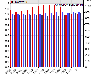

In this case the optimizer would select a parameter value of about 1.3 for the sine phase and about 1.0 (not the peak at 0.9) for the amplitude threshold for the current asset (EUR/USD). The exit time is not optimized in this step, as we’ll do that later together with the other exit parameters when risk management is implemented.
Step 6: Out-of-sample analysis
Of course the parameter optimization improved the backtest performance of the strategy, since the system was now better adapted to the price curve. So the test result so far is worthless. For getting an idea of the real performance, we first need to split the data into in-sample and out-of-sample periods. The in-sample periods are used for training, the out-of-sample periods for testing. The best method for this is Walk Forward Analysis. It uses a rolling window into the historical data for separating test and training periods.
Unfortunately, WFA adds two more parameters to the system: the training time and the test time of a WFA cycle. The test time should be long enough for trades to properly open and close, and small enough for the parameters to stay valid. The training time is more critical. Too short training will not get enough price data for effective optimization, training too long will also produce bad results since the market can already undergo changes during the training period. So the training time itself is a parameter that had to be optimized.
A five cycles walk forward analysis (add “NumWFOCycles = 5;” to the above script) reduces the backtest performance from 100% annual return to a more realistic 60%. For preventing that WFA still produces too optimistic results just by a lucky selection of test and training periods, it makes also sense to perform WFA several times with slightly different starting points of the simulation. If the system has an edge, the results should be not too different. If they vary wildly: back to step 3.
Step 7: Reality Check
Even though the test is now out-of-sample, the mere development process – selecting algorithms, assets, test periods and other ingredients by their performance – has added a lot of selection bias to the results. Are they caused by a real edge of the system, or just by biased development? Determining this with some certainty is the hardest part of strategy development.
The best way to find out is White’s Reality Check. But it’s also the least practical because it requires strong discipline in parameter and algorithm selection. Other methods are not as good, but easier to apply:
- Montecarlo. Randomize the price curve by shuffling without replacement, then train and test again. Repeat this many times. Plot a distribution of the results (an example of this method can be found in chapter 6 of the Börsenhackerbuch). Randomizing removes all price anomalies, so you hope for significantly worse performance. But if the result from the real price curve lies not far east of the random distribution peak, it is probably also caused by randomness. That would mean: back to step 3.
- Variants. It’s the opposite of the Montecarlo method: Apply the trained system on variants of the price curve and hope for positive results. Variants that maintain most anomalies are oversampling, detrending, or inverting the price curve. If the system stays profitable with those variants, but not with randomized prices, you might really have found a solid system.
- Really-out-of-sample (ROOS) Test. While developing the system, ignore the last year (2015) completely. Even delete all 2015 price history from your PC. Only when the system is completely finished, download the data and run a 2015 test. Since the 2015 data can be only used once this way and is then tainted, you can not modify the system anymore if it fails in 2015. Just abandon it. Assemble all your metal strength and go back to step 1.
Step 8: Risk management
Your system has so far survived all tests. Now you can concentrate on reducing its risk and improving its performance. Do not touch anymore the entry algorithm and its parameters. You’re now optimizing the exit. Instead of the simple timed and reversal exits that we’ve used during the development phase, we can now apply various trailing stop mechanisms. For instance:
- Instead of exiting after a certain time, raise the stop loss by a certain amount per hour. This has the same effect, but will close unprofitable trades sooner and profitable trades later.
- When a trade has won a certain amount, place the stop loss at a distance above the break even point. Even when locking a profit percentage does not improve the total performance, it’s good for your health. Seeing profitable trades wander back into the losing zone can cause serious ulcers.
This is our example script with the initial timed exit replaced by a stop loss limit that rises at every bar:
function run()
{
  vars Price = series(price());
  var Phase = DominantPhase(Price,10);
  vars Signal = series(sin(Phase+optimize(1,0.7,2)*PI/4));
  vars Dominant = series(BandPass(Price,rDominantPeriod,1));
  var Threshold = optimize(1,0.7,2)*PIP;

  Stop = ATR(100);
  for(open_trades)
    TradeStopLimit -= TradeStopDiff/(10*rDominantPeriod);

  if(Amplitude(Dominant,100) > Threshold) {
    if(valley(Signal))
      reverseLong(1);
    else if(peak(Signal))
      reverseShort(1);
  }
}
The for(open_trades) loop increases the stop level of all open trades by a fraction of the initial stop loss distance at the end of every bar.
Of course you now have to optimize and run a walk forward analysis again with the exit parameters. If the performance didn’t improve, think about better exit methods.
Step 9: Money management
Money management serves three purposes. First, reinvesting your profits. Second, distributing your capital among portfolio components. And third, quickly finding out if a trading book is useless. Open the “Money Management” chapter and read the author’s investment advice. If it’s “invest 1% of your capital per trade”, you know why he’s writing trading books. He probably has not yet earned money with real trading.
Suppose your trade volume at a given time t is V(t). If your system is profitable, on average your capital C will rise proportionally to V with a growth factor c:
\frac{dC}{dt} = c V(t)~~\rightarrow~~ C(t) = C_0 + c \int_{0}^{t}{V(t) dt}When you follow trading book advices and always invest a fixed percentage p of your capital, so that V(t) = p C(t), your capital will grow exponentially with exponent p c:
\frac{dC}{dt} ~=~ c p C(t) ~~\rightarrow~~ C(t) ~=~ C_0 e^{p c t}Unfortunately your capital will also undergo random fluctuations, named Drawdowns. Drawdowns are proportial to the trade volume V(t). On leveraged accounts with no limit to drawdowns, it can be shown from statistical considerations that the maximum drawdown depth Dmax grows proportional to the square root of time t:
{D_{max}}(t) ~=~ q V(t) \sqrt{t}So, with the fixed percentage investment:
{D_{max}}(t) ~=~ q p C(t) \sqrt{t}and at the time T = 1/(q p)2:
{D_{max}}(T) ~=~ q p C(T) \frac{1}{q p} ~=~ C(T)You can see that around the time T = 1/(q p)2 a drawdown will eat up all your capital C(T), no matter how profitable your strategy is and how you’ve choosen p! That’s why the 1% rule is a bad advice. And why I advise clients not to raise the trade volume proportionally to their accumulated profit, but to its square root – at least on leveraged accounts. Then, as long as the strategy does not deteriorate, they keep a safe distance from a margin call.
Dependent on whether you trade a single asset and algorithm or a portfolio of both, you can calculate the optimal investment with several methods. There’s the OptimalF formula by Ralph Vince, the Kelly formula by Ed Thorp, or mean/variance optimization by Harry Markowitz. Usually you won’t hard code reinvesting in your strategy, but calculate the investment volume externally, since you might want to withdraw or deposit money from time to time. This requires the overall volume to be set up manually, not by an automated process. A formula for proper reinvesting and withdrawing can be found in the Black Book.
Step 10: Preparation for live trading
You can now define the user interface of your trading system. Determine which parameters you want to change in real time, and which ones only at start of the system. Provide a method to control the trade volume, and a ‘Panic Button’ for locking profit or cashing out in case of bad news. Display all trading relevant parameters in real time. Add buttons for re-training the system, and provide a method for comparing live results with backtest results, such as the Cold Blood Index. Make sure that you can supervise the system from whereever you are, for instance through an online status page. Don’t be tempted to look onto it every five minutes. But you can make a mighty impression when you pull out your mobile phone on the summit of Mt. Ararat and explain to your fellow climbers: “Just checking my trades.”
The real strategy development
So far the theory. All fine and dandy, but how do you really develop a trading system? Everyone knows that there’s a huge gap between theory and practice. This is the real development process as testified by many seasoned algo traders:
Step 1. Visit trader forums and find the thread about the new indicator with the fabulous returns.
Step 2. Get the indicator working with a test system after a long coding session. Ugh, the backtest result does not look this good. You must have made some coding mistake. Debug. Debug some more.
Step 3. Still no good result, but you have more tricks up your sleeve. Add a trailing stop. The results now look already better. Run a week analysis. Tuesday is a particular bad day for this strategy? Add a filter that prevents trading on Tuesday. Add more filters that prevent trades between 10 and 12 am, and when the price is below $14.50, and at full moon except on Fridays. Wait a long time for the simulation to finish. Wow, finally the backtest is in the green!
Step 4. Of course you’re not fooled by in-sample results. After optimizing all 23 parameters, run a walk forward analysis. Wait a long time for the simulation to finish. Ugh, the result does not look this good. Try different WFA cycles. Try different bar periods. Wait a long time for the simulation to finish. Finally, with a 19-minutes bar period and 31 cycles, you get a sensational backtest result! And this completely out of sample!
Step 5. Trade the system live.
Step 6. Ugh, the result does not look this good.
Step 7. Wait a long time for your bank account to recover. Inbetween, write a trading book.
I’ve added the example script to the 2016 script repository. In the next part of this series we’ll look into the data mining approach with machine learning systems. We will examine price pattern detection, regression, neural networks, deep learning, decision trees, and support vector machines.
I smell a book written by Italians….
Thanks for a great series of articles – I’m looking forward to testing out the concepts you’ve discussed. However, I failed at the first hurdle when I noticed my frequency spectrum over October 2015 didn’t match yours. Then I noticed the EURUSD spectrum says XAGUSD in the corner 🙂
Indeed, seems I’ve uploaded the wrong image.
WOW, look forward to the upcoming articles. You do such a great job condensing a great deal of info into simple and easy to read articles.
This is probably one of the best post and most important post I have read in the field. I have read some books about strategy development which are not as good as this post. You could write a book hehe … but I see you dont which means you win 🙂
These are great articles. Thank you.
I’m curios to understand beside these modeling strategies, are you aware of quantitative strategies that takes into consideration broader set of more diverse datasets, like looking at economic indicators or social sentiment and combining with historical prices of different assets categories.
Yes. We did a couple model-based systems for clients that got additional information from the VIX or the COTR. I cannot say that using these datasets drastically improved profits, but in some cases they worked well for filters or for determining trend.
Dear Jcl, thank you so much for this blog and for your efforts in the Zorro community. I am just approaching it, and it looks like this could be really the environment where > 10 years of “puzzled” research come together!
This post is very fine, but I would ask you to go into some details about at least one point. You say: “The precise performance does not matter much at this point – just determine whether the algorithm has an edge or not”. How do you define and measure this edge? You might agree this is no trivial question, and you teach me how many ways there are to define and measure it (somebody suggesting to make it at the “signal” rather than “entry” level, see Peterson…).
For instance, if you apply your very first script to EURUSD, 1H, from 2011 to 2015, you get in the performance result a 0.98 profit factor, and average yearly loss of 5%, a Sharpe of -0.16. How do you decide to go on with research? Which are the parameters that you suggest for the first backtests? Is there a parameter-less measure of the edge? Is a SAR “system” really the best set-up for measuring edge, or this comes for instance by the application of an indicator/signal/entry logic + a filter?
These questions are where, due to the “combinatorial complexity” of possibilities (and theories around) I still start driving into the fog…
Thank you so much!
This is a good question. You’ll normally write an algorithm step by step, from a first simple and raw version to the final version. At some point you have to decide whether to continue, or go back and try different ways. So you’re permanently backtesting variants. You will not necessarily get good total profits at first. But when the method has an edge, it should at least be profitable in certain market periods and situations. That’s the periods and situations that you then analyze in more detail, for finding out why your algorithm works there and not elsewhere, and how you could detect them or filter them out.
There is no simple formula, every algorithm has a different approach. The same inefficiency can be exploited with thousands of different algorithms. Maybe 90% them do not work at all because they react to slow or are too sensitive to noise or for other reasons. You must always be prepared to abandon an algorithm when you can not find at least a temporary clear edge within a reasonable amount of time.
Thank you Jcl, very useful.
I am still puzzled, though. Surely your good systems could provide a benchmark for testing some of the measures around, like the e-ratio by C. Faith, or the “acrary edge test”, and perhaps still more (information gain and the like). I think that some statistic about “signals” (before going into rules, see again Peterson) could be very valuable, also when for instance looking into data mining for finding inefficiencies. Zorro seems the ideal environment for making such tests. And, perhaps you would agree, if we want to be strict and a bit “scientific”, we should try to avoid the use of “fat words” like “edge”, if we cannot measure it.
But your “hacker” approach seems very sound and productive (more than analysis paralysis, which is often my problem, surely!).
Really enjoyed this series of articles, thanks man!
Just an FYI, for more complex parameter optimization problems I would consider multimodal global optimization algorithms over unimodal local optimization algorithms because of the characteristics of the fitness landscape and the presence non stationarity optima / regimes 🙂
This is a different philosophy of parameter optimization. Multimodal optimization finds a local maximum in an irregular fitness landscape, while unimodal optimization finds the global maximum in a rather regular landscape. Clearly, the former gets higher performance in backtests. But the question is if a system will be robust and profitable in real trading when it has an irregular fitness landscape and was optimized at a local peak. I think: no. But this would be indeed an interesting question to check out, and maybe the topic of a future study and blog post.
jcl – First off, congrats on developing quality content! I am fortunate enough to have stumbled into this and it’s going to keep me busy for sometime. One question (among many others 🙂 I have.
You say “But do not yet use any stops, trailing, or other bells and whistles. They would only distort the result..”. In my backtests of an intraday trading system, I am using fixed stop loss and profit target and is an outcome from every training interval. My assumption was, these tie into the ADR (daily range or volatility) of the recent market conditions and hence should be tuned. However, I would love to hear your inputs on this and if this creates more curve fitting risk that I don’t see.
Thanks again for putting this altogether!
Yes, you can and should absolutely use volatility dependent stops and tune them. But I suggest not to do that in the early stage when you just want to find out if your algorithm works at all. Tuning and complex exits just makes it more difficult to decide if there really is an “edge”, or “alpha”, or “truth”, or whatever you call it, to your entry algorithm.
Hi,
Do you have any news about the following (a dead link):
Hello ,
a new article was posted on the Financial Hacker blog:
Build Better Strategies! Part 4: Data Mining
In 1996, Deep Blue was the first computer to win the chess championship. It took 20 more years until the leading Go player Lee Sedol was defeated by a computer program, AlphaGo. Deep Blue was a model based system with hardwired chess rules. AlphaGo is a data-mining system, a deep …
You can view it at http://www.financial-hacker.com/build-better-strategies-part-4-data-mining/.
You received this e-mail because you asked to be notified when new articles are posted.
Thanks & Best Regards!
The Financial Hacker
Sorry for that – it was an email glitch by hitting a wrong button. I had started the article, but then something came up and I had not yet the time to finish it. But I’ll do that soon.
Hi
I did the Really-out-of-sample (ROOS) Test with 2015 historical data. My PF>1 and SR~<1 and it give 2000pips at the end of the year. However the equity curve is flat with R=0.00.
I dont know if it make sense to go back to step 1 and try to improve R with risk control or if such a result is an indicator that my strategy has no edge from the beginning. I know it is dificult to say with just such info but I just wonder as a global question how bad or how go the ROOS has to be to keep using the strategy or to abandon it. Maybe the rule is that the strategy has to give the same results during 2015 as the backtest during the whole 2014?
The R2 value is not really relevant here, since R2 is a long-term parameter that needs a longer equity curve than only one year. There are two other questions that a ROOS test can answer: Does the result look very different to the results from any year before? And would you have started trading this system in January when you knew the end result in December?
Good to know that R2 isnt that important. 🙂
These are actually really good questions. Even Z12 taken a bad year can look not that good to go live with it. My DD, PF and MI and SR of the year in the ROOS are similar to the backtest result because there is also a flat period on the backtest too which produces similar DD. The question is if this flat period will keep on going and since I dont know yet how to filter it, it is like throwing a coin to go life. Could it be possible to use Cold Blood Index during the ROOS?
Yes, the CBI works for the ROOS period just as for live trading. The long flat periods are due to the filter – it’s not optimal here. This is not a commercial quality system, it’s only for demonstration.
Thanks for the answer.
I have an extrange situation now tho. My strategy past the ROOS test for the assets I prepare in the training period but I do not have any parameters optimized because I want to control the number of pips on risk per trade. However if I apply WFO then it is a disaster ( or almost ). On one side it can be due to overfitting ofc but then I do not know how the strategy can pass ROSS. On the other side I noticed in the performance report a big unbalance between long and short trades after the WFO. It looks like the most stable PF is obtained for a parameter value which actually produces only trades in one direcction and at the end, the result isnt that good. Can detrend solve that problem? Should the training consider the PF stability of long and short trades?
If I understood you right, your strategy passed the ROOS test with default parameters, but after optimizing with WFO it failed. The ROOS test must be done after WFO, not before. Otherwise it can be just a lucky selection of parameter default values. A long/short asymmetry after WFO is probably an artifact caused by a strong trend during the training periods. In that case you should indeed detrend the trade results in training.
Yes thats correct. I did not do WFO or parameter optimization the first time and I prepared the strategy so but then I begun again with a WFO to compare the strategies and in that case I got such a bad result. It is good to know that ROOS has to be done after WFO and that WFO is mandatory.
I detrended it and the problem was still there. It was indeed an artifact because I found out that the trades were placed in the wrong side for some of the assets due to a too big rollover so I probably updated the asset list on a wrong day
Nice article. Just beginning my algorithmic trading journey and I often refer back to this article when developing. You mention that “Your algorithm must be able to produce positive returns either with pure reversal, or at least with a timed exit.”
It seems that the suggestion here is to leave the trade after a reversal is detected, or when, let’s say, n candles have passed since the entry of the trade. Is this not highly dependent on how you define 1) a reversal and 2) the size n?
It seems that this too also introduces some selection bias into the initial steps of developing an algorithm.
No, with “reversal” I mean a trade reversal, not a price reversal. The algorithm opens a short trade, and this closes a long position, or vice versa. Most algorithms are symmetric, so they can go long or short.
Exceptions are long-only strategies for stocks or ETFs. They do not reverse, so you need some other means for closing a trade. In most cases the algorithm still produces a native close signal that is the opposite of the open signal. If not, you must use a timed exit. For determining n, you normally plot a price profile at trade entry. Zorro has a function for plotting such a profile. n is then a point after the price turns back.
Jcl thanks for the prompt reply!
It looks like a simple straight forward process. Find an indicator which gives a SR>1 on a test with a simple script in some assets and you are ready to go. The question could be: Is there a certain minimun amount of assets which have to give good results with the simple script in order to ensure that it has an edge or is it enough if just one/two/three assets produce good results?
I said that the process looks simple because it gets kind of more complicate when more assets and algos has to be added. In the tutorial it is written that at least 10 algos and 10 assets have to be combined in order to create a robuts strategy. I struggle in this part because eventhough I can find some algos which behave ok with the reversal script, I am not sure what is the right way to proceed when it is time to combine them.
Has this step-by-step framework protocol been empirically studied to determine its efficacy/reliability? How many systems generated and undergone such robustness tests using the whole procedure described above, have turned out to be profitable under live forward tests (and for how long)? Can we quantify all the results of the number of systems that failed these tests vs. the number of systems that have passed? Are there verified real accounts to provide evidence of efficacy for this particular framework? Has anybody attempted to compare this framework to Michael Harris’ [advertisement link removed]?
Please, advertise your software on your own website, not on my blog. Thank you. – Assuming the question was serious: This article is not about a new invented “framework” for trade systems, or something like that. I’m describing the standard process of building a software model. This works in a similar way with any predictive model, not necessarily for trading.
Nice article, thanks JCL. Just one note on money management. According to Magdon-Ismail scaling of the expected MDD with T undergoes a phase transition from T to √T to log T as µ changes from negative to zero to positive. A drawdown will eat up all your capital C(T) at some time, but it’ll take more time. For example for a system with Kelly 12.5 it won’t take 40 years (for √T scaling) but something like 1 million years (for log T scaling).
Peter
This is correct; in the strong sense the √T scaling is only valid for systems with neither positive nor negative expectancy. But there are more factors involved. Magdon-Ismail considered a drift term µ > 0, which increases the time until crash, but did not consider a (very likely) autocorrelation of the results, which reduces the time until crash. So with assuming a √T scaling you’re more on the safe side than with log T.
jcl,
I’ve been following your blog and reading old blog posts (and re-reading them) as I’ve started dedicating more time to algorithmic trading. I like the way you write and explain things, it’s clear and just the right amount of detail. Thank you.
Beginner question on Research and Algorithm steps. When developing a strategy that uses a classifier to detect discrete occurrences (rather than time-series patterns), is it appropriate to use standard/randomized cross-validation for algorithm evaluation and optimization? Or should we be doing these iterative improvements on the WFA? I’ve been getting good results with CV but WFA clearly shows higher variability between cycles.
Cheers,
RJ
In my opinion CV is not well suited for nonstationary time series. Its advantage, more data, is outweighed by its disadvantage, peeking bias. The problem is that a part of the training data is from the future. So a future trend or other market change has effect on the test result, which might be too positive when that trend was just beginning in the test period. WFA simulates better the real trading situation where training data is always from the past. And high variability is what you indeed experience when you trade an algorithmic system live.
Hi jcl,
Another quick question if you don’t mind.
What is the proper way of dealing with trades/samples that are overlapping 2 WFA cycles?
For example, I am looking into placing trades on daily timeframe and retraining the model monthly. Inevitably, some trades will be started in one WFA test cycle and will still be open in the next cycle when that particular trade becomes a part of the training dataset.
Just count them in the test results in which WFA cycle they finish and not use it in the training set until the trade closes? This would skew the test results, but at least it would mimic real life. Any thoughts?
Thank you.
The proper way is to have a ‘horizon’ period between the end of the training cycle and the start of the test cycle. Zorro has a variable for this, DataHorizon, but you can do this relatively easily also in other platforms by counting the test cycle bars and not opening trades until the maximum overlap period is over.
Your idea of filtering trades by finding the dominant cycle period to the price curve and measuring its amplitude is interesting.Another idea might be that Dr. Claudio Antonini’s the Q-Gaussian distribution works in econometrics.His papers are no longer available on the net but according to article in here https://www.mql5.com/en/articles/412 the Q-Gaussian distributions fit the instrument( technical analysis)/timeframe dependence well.What do you think?
Since price distribution is often not Gaussian, many other distributions have been proposed to better model prices, so why not the Q-Gaussian. This looks like an interesting approach. I’ll check it out. Thanks for the link.
Good stuff. Working here. Thank you.
Is there a trading strategy with backtests/code available that employ hidden markov models and baum welch/viterbi algorithm ?
No, but you can write such a strategy. Or hire us to do it.
I am looking for a portfolio management script with Al and well as with manual trading leader to the follower. (trade copy engine) with strict risk management control applied to the traders ( you can say prop trading) irrespective of this trading style with machine learning and adopt his style of trading with due course of time. please let me know how much will it cost.
How much it will cost depends on the details of the system. You can contact my colleagues at info@opgroup.de and discuss the project.
Got very poor predictability from using these ExploitCycles in ML model . Very low close to random. This does not seem to detect cycles in holdout data, meaning this does not generalize very well at all